Fine-mapping and LD diagnosis with UK Biobank reference LD matrices
Kaixuan Luo
Source:vignettes/finemapping_ukbb_ld_diagnosis.Rmd
finemapping_ukbb_ld_diagnosis.RmdIn this tutorial, we show an example of performing fine-mapping and LD mismatch diagnosis (using susie_rss) with pre-computed LD matrices from UK Biobank reference.
We have pre-computed the LD matrices of European samples from UK Biobank. They can be downloaded here.
Load the packages.
Load an example Asthma GWAS summary statistics
gwas.file <- '/project2/xinhe/shared_data/mapgen/example_data/GWAS/aoa_v3_gwas_ukbsnps_susie_input.txt.gz'
gwas.sumstats <- vroom::vroom(gwas.file, col_names = TRUE, show_col_types = FALSE)
head(gwas.sumstats)
## # A tibble: 6 × 10
## chr pos beta se a0 a1 snp pval zscore locus
## <dbl> <dbl> <dbl> <dbl> <chr> <chr> <chr> <dbl> <dbl> <dbl>
## 1 1 693731 0.00277 0.0156 A G rs12238997 0.859 0.178 1
## 2 1 707522 0.00337 0.0169 G C rs371890604 0.841 0.200 1
## 3 1 717587 -0.0538 0.0429 G A rs144155419 0.210 -1.25 1
## 4 1 723329 0.00182 0.128 A T rs189787166 0.989 0.0143 1
## 5 1 729679 0.00577 0.0142 C G rs4951859 0.684 0.407 1
## 6 1 730087 -0.00465 0.0220 T C rs148120343 0.832 -0.212 1
n = 336210Load LD blocks
LD_Blocks <- readRDS(system.file('extdata', 'LD.blocks.EUR.hg19.rds', package='mapgen'))Obtain a data frame of region_info, rows are LD block coordinates together with the filenames of UKBB reference LD matrices and SNP info.
region_info <- get_UKBB_region_info(LD_Blocks,
                                    LDREF.dir = "/project2/mstephens/wcrouse/UKB_LDR_0.1_b37",
                                    prefix = "ukb_b37_0.1")
Read all SNP info from the LD reference
LD_snp_info <- read_LD_SNP_info(region_info)Process GWAS summary statistics and add LD block information, harmonize GWAS summary statistics with LD reference, flip signs when reverse complement matches and remove strand ambiguous variants
gwas.sumstats <- process_gwas_sumstats(gwas.sumstats,
                                       chr='chr', pos='pos', beta='beta', se='se',
                                       a0='a0', a1='a1', snp='snp', pval='pval',
                                       LD_snp_info=LD_snp_info,
                                       strand_flip=TRUE,
                                       remove_strand_ambig=TRUE)
## Cleaning summary statistics...
## Harmonizing GWAS SNPs with LD reference panel...
## 9732903 variants in sumstats before harmonization...
## 6419678 variants in both sumstats and LD reference ...
## Flip signs for 6419677 (100.00%) variants with allele flipped.
## Remove 994657 (18.33%) strand ambiguous variants.Select GWAS significant loci (pval < 5e-8)
if (max(gwas.sumstats$pval) > 1) {
  gwas.sumstats <- gwas.sumstats %>% dplyr::mutate(pval = 10^(-pval))
}

sig.loci <- gwas.sumstats %>% dplyr::filter(pval < 5e-8) %>% dplyr::pull(locus) %>% unique()
cat(length(sig.loci), "significant loci. \n")
## 17 significant loci.Fine-mapping
Fine-mapping significant loci with pre-computed UKBB LD matrices (we use uniform prior in this tutorial).
If we set save = TRUE, it saves susie result as well as z-scores and R matrix for each locus, which could be used later for diagnosis.
selected.sumstats <- gwas.sumstats[gwas.sumstats$locus %in% sig.loci, ]

susie.results <- run_finemapping(selected.sumstats,
                                 region_info = region_info,
                                 priortype = 'uniform', n = n, L = 10,
                                 save = TRUE, outputdir = "./test", outname = "example")

susie.sumstats <- merge_susie_sumstats(susie.results, sumstats.locus)
run_finemapping() internally runs susie_finemap_region() for each of the loci. For finemapping a single locus, we can simply use susie_finemap_region() with sumstats and LD information (R and snp_info) for the locus.
locus <- sig.loci[2]
sumstats.locus <- gwas.sumstats[gwas.sumstats$locus == locus, ]

# load LD matrix and SNP info for this locus
LD_ref <- load_UKBB_LDREF(LD_Blocks,
                          locus,
                          LDREF.dir = "/project2/mstephens/wcrouse/UKB_LDR_0.1_b37",
                          prefix = "ukb_b37_0.1")

# Match GWAS sumstats with LD reference, only keep variants included in LD reference.
matched.sumstat.LD <- match_gwas_LDREF(sumstats.locus, LD_ref$R, LD_ref$snp_info)
sumstats.locus <- matched.sumstat.LD$sumstats
z.locus <- sumstats.locus$zscore
R.locus <- matched.sumstat.LD$R
snp_info.locus <- matched.sumstat.LD$snp_info

susie.locus.res <- susie_finemap_region(sumstats.locus, R.locus, snp_info.locus, n = n, L = 10)
## Run susie_rss...
susieR::susie_plot(susie.locus.res, y='PIP')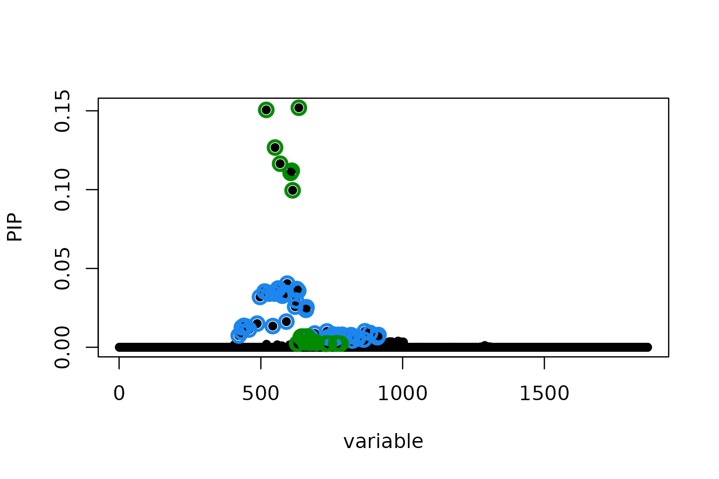
susie.locus.sumstats <- merge_susie_sumstats(susie.locus.res, sumstats.locus)LD mismatch diagnosis
Inconsistencies between GWAS z-scores and the LD reference could potentially inflate PIPs from SuSiE finemapping when L > 1. It would be helpful to check for potential LD mismatch issues, for example using DENTIST or susie_rss.
Here we perform LD mismatch diagnosis for this example locus using susie_rss:
condz <- LD_diagnosis_susie_rss(z.locus, R.locus, n)## Estimate consistency between the z-scores and reference LD matrix ...
## Estimated lambda = 7.30936e-05
## Compute expected z-scores based on conditional distribution of z-scores ...
condz$plot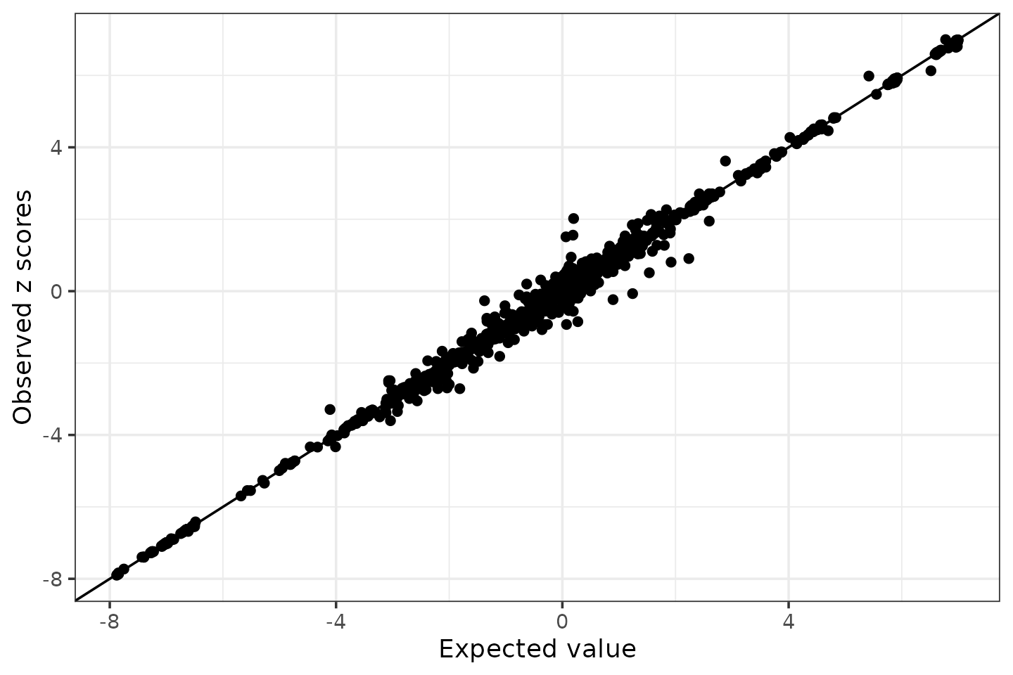
The estimated lambda is very small, and the LD mismatch diagnosis plot looks good (with no allele flipping detected), which suggests that the GWAS z-scores and reference LD are consistent.
Next, we manually introduces LD mismatches by flipping alleles for 10 variants (with large effects) and see if we can detect those.
seed = 1
set.seed(seed)

flip_index <- sample(which(sumstats.locus$zscore > 2), 10)
sumstats.locus.flip <- sumstats.locus
sumstats.locus.flip$zscore[flip_index] <- -sumstats.locus$zscore[flip_index]

cat(length(flip_index), "allele flipped variants:\n", sort(sumstats.locus.flip$snp[flip_index]), "\n")
## 10 allele flipped variants:
## rs10184597 rs10189629 rs10203707 rs10207579 rs13392285 rs2110727 rs2215945 rs62154973 rs72823628 rs72823646Then, we run fine-mapping including variants with flipped alleles.
susie.results <- run_finemapping(sumstats.locus.flip, region_info = region_info, priortype = 'uniform', n = n, L = 10)## Finemapping 1 loci...
## Finemapping locus 193...
## Run susie_rss...
susie.locus.res <- susie.results[[1]]
susieR::susie_plot(susie.locus.res, y='PIP')
Let’s compare observed z-scores vs the expected z-scores.
condz <- LD_diagnosis_susie_rss(sumstats.locus.flip$zscore, R = R.locus, n = n)## Estimate consistency between the z-scores and reference LD matrix ...
## Estimated lambda = 0.4730198
## Compute expected z-scores based on conditional distribution of z-scores ...
# condz$plotDetect possible allele flipped variants (logLR > 2 and abs(z) > 2).
detected_index <- which(condz$conditional_dist$logLR > 2 & abs(condz$conditional_dist$z) > 2)
cat(sprintf("Detected %d variants with possible allele flipping", length(detected_index)), "\n")
## Detected 10 variants with possible allele flipping## Possible allele switched variants: rs10184597 rs10189629 rs10203707 rs10207579 rs13392285 rs2110727 rs2215945 rs62154973 rs72823628 rs72823646
condz$conditional_dist$flipped <- 0
condz$conditional_dist$flipped[flip_index] <- 1
condz$conditional_dist$detected <- 0
condz$conditional_dist$detected[detected_index] <- 1

cat(sprintf("%d out of %d flipped variants detected with logLR > 2 and abs(z) > 2. \n",
            length(intersect(detected_index, flip_index)), length(flip_index)))
## 10 out of 10 flipped variants detected with logLR > 2 and abs(z) > 2.
condz$conditional_dist[union(flip_index, detected_index),]## z condmean condvar z_std_diff logLR flipped detected
## 529 -6.965514 6.321319 0.4847394 -19.083908 8.381969 1 1
## 1065 -2.567840 2.471008 0.4833665 -7.247579 8.078109 1 1
## 836 -2.532926 2.380152 0.4935893 -6.993116 8.042908 1 1
## 1048 -2.611843 2.493572 0.4837408 -7.340484 8.074479 1 1
## 218 -3.510579 3.281118 0.5026859 -9.579216 8.133171 1 1
## 115 -4.280961 4.094475 0.4988993 -11.857713 8.320665 1 1
## 1365 -3.318277 3.265362 0.5069206 -9.246898 8.196465 1 1
## 433 -6.686770 6.123010 0.4997885 -18.119598 8.451238 1 1
## 624 -6.934847 6.350230 0.4841194 -19.093601 8.509518 1 1
## 142 -4.512544 4.337933 0.4937149 -12.595882 8.385750 1 1
ggplot(condz$conditional_dist, aes(x = condmean, y = z, col = factor(flipped))) +
  geom_point() +
  scale_colour_manual(values = c("0" = "black", "1" = "red")) +
  labs(x = "Expected value", y = "Observed z scores", color = "Simulated allele flipping") +
  theme_bw()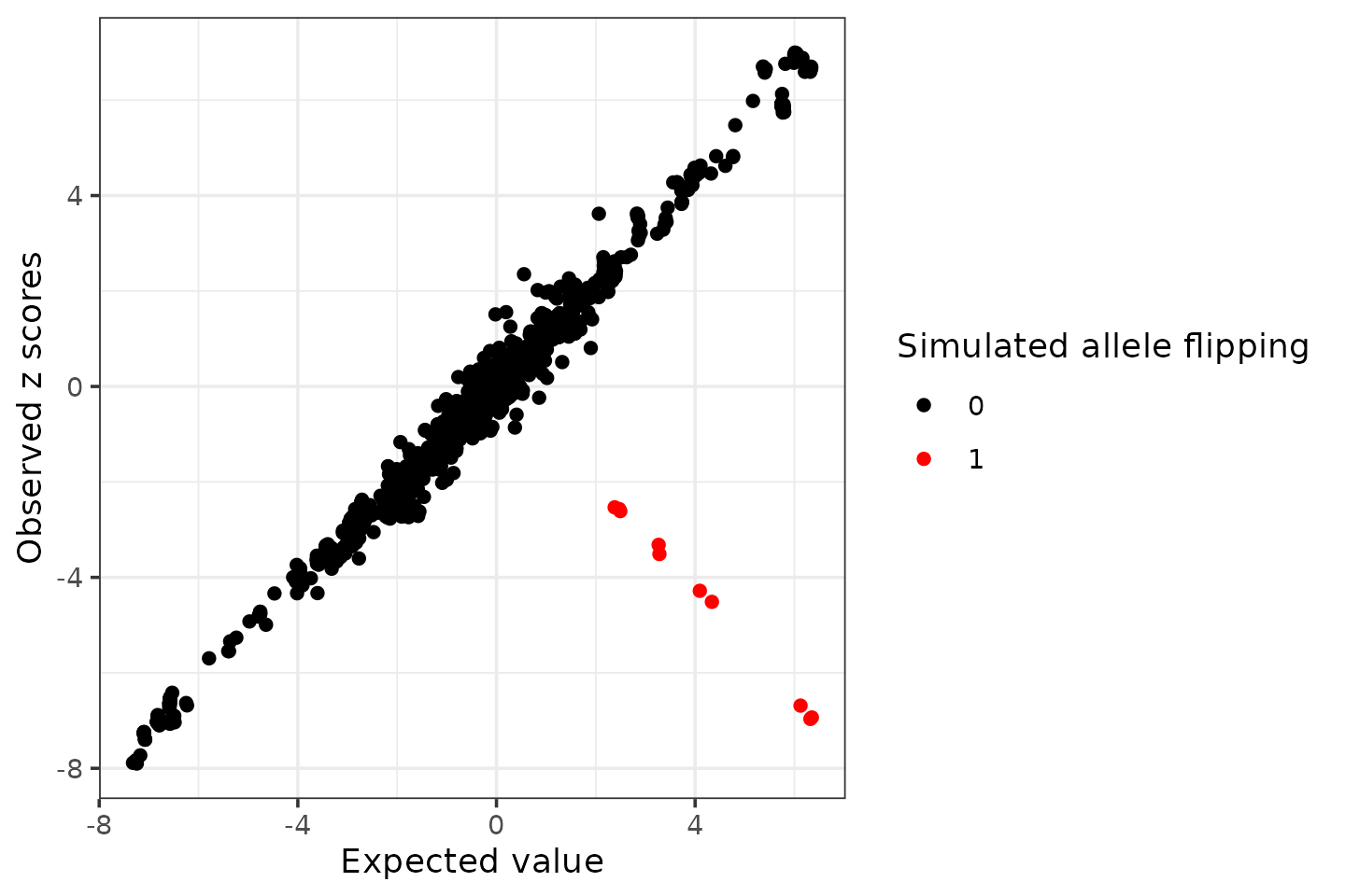
ggplot(condz$conditional_dist, aes(x = condmean, y = z, col = factor(detected))) +
  geom_point() +
  scale_colour_manual(values = c("0" = "black", "1" = "red")) +
  labs(x = "Expected value", y = "Observed z scores", color = "Detected allele flipping") +
  theme_bw()