Enrichment analysis using mapgen
Kaixuan Luo
2022-04-11
Last updated: 2023-10-20
Checks: 7 0
Knit directory: analysis_pipelines/
This reproducible R Markdown analysis was created with workflowr (version 1.7.0). The Checks tab describes the reproducibility checks that were applied when the results were created. The Past versions tab lists the development history.
Great! Since the R Markdown file has been committed to the Git repository, you know the exact version of the code that produced these results.
Great job! The global environment was empty. Objects defined in the global environment can affect the analysis in your R Markdown file in unknown ways. For reproduciblity it’s best to always run the code in an empty environment.
The command set.seed(20200524) was run prior to running
the code in the R Markdown file. Setting a seed ensures that any results
that rely on randomness, e.g. subsampling or permutations, are
reproducible.
Great job! Recording the operating system, R version, and package versions is critical for reproducibility.
Nice! There were no cached chunks for this analysis, so you can be confident that you successfully produced the results during this run.
Great job! Using relative paths to the files within your workflowr project makes it easier to run your code on other machines.
Great! You are using Git for version control. Tracking code development and connecting the code version to the results is critical for reproducibility.
The results in this page were generated with repository version 79c858f. See the Past versions tab to see a history of the changes made to the R Markdown and HTML files.
Note that you need to be careful to ensure that all relevant files for
the analysis have been committed to Git prior to generating the results
(you can use wflow_publish or
wflow_git_commit). workflowr only checks the R Markdown
file, but you know if there are other scripts or data files that it
depends on. Below is the status of the Git repository when the results
were generated:
Ignored files:
    Ignored:    .Rhistory
    Ignored:    .Rproj.user/

Untracked files:
    Untracked:  analysis/test_sldsc_splicingAnnot.Rmd
    Untracked:  code/compute_ldscore_generic_annot.sbatch
    Untracked:  code/extract_baselineLD_generic_annot.R
    Untracked:  code/ldsc_make_binary_annot_compute_ldscores_bedfiles.sbatch
    Untracked:  code/make_ldsc_binary_annots_from_bedfiles.R
    Untracked:  code/sldsc_annot_generic_baselineLD_separate.sbatch
    Untracked:  scripts/tmp.R

Unstaged changes:
    Modified:   analysis/index.Rmd
    Modified:   analysis/mapgen_torus_susie_AF.Rmd
    Modified:   analysis/sldsc_example_GTEx_QTLs.Rmd
    Modified:   analysis/sldsc_pipeline.Rmd
    Modified:   code/extract_baselineLDv2.2_generic_annot.R
    Modified:   code/mapgen_trackplots.R
    Modified:   scripts/run_finemapping.R
Note that any generated files, e.g. HTML, png, CSS, etc., are not included in this status report because it is ok for generated content to have uncommitted changes.
These are the previous versions of the repository in which changes were
made to the R Markdown
(analysis/mapgen_torus_enrichment_heart_atlas.Rmd) and HTML
(docs/mapgen_torus_enrichment_heart_atlas.html) files. If
you’ve configured a remote Git repository (see
?wflow_git_remote), click on the hyperlinks in the table
below to view the files as they were in that past version.
| File | Version | Author | Date | Message |
|---|---|---|---|---|
| Rmd | 79c858f | kevinlkx | 2023-10-20 | wflow_publish("analysis/mapgen_torus_enrichment_heart_atlas.Rmd") |
| html | 0d76d5c | kevinlkx | 2022-04-22 | Build site. |
| Rmd | cb7333c | kevinlkx | 2022-04-22 | fixed bugs in run_torus() |
| html | ce62d73 | kevinlkx | 2022-04-22 | Build site. |
| Rmd | 4bcdf12 | kevinlkx | 2022-04-22 | fixed bugs in run_torus() return values and added torus_input_dir for prepare_torus_input_files() |
| html | db1ff60 | kevinlkx | 2022-04-19 | Build site. |
| Rmd | 39e9a66 | kevinlkx | 2022-04-19 | wflow_rename("analysis/torus_enrichment_heart_atlas.Rmd", "analysis/mapgen_torus_enrichment_heart_atlas.Rmd") |
| html | 39e9a66 | kevinlkx | 2022-04-19 | wflow_rename("analysis/torus_enrichment_heart_atlas.Rmd", "analysis/mapgen_torus_enrichment_heart_atlas.Rmd") |
Here we show an example of performing enrichment analysis on AFib
GWAS data using mapgen.
Univariate enrichment analysis
Here we use scATAC-seq DA peaks as annotations (univariate).
library(mapgen)
library(tidyverse)
suppressMessages(library(liftOver))
suppressMessages(library(ComplexHeatmap))
data.dir <- '/project2/xinhe/shared_data/mapgen/example_data'Load GWAS summary statistics of AFib
gwas.sumstats <- readRDS(paste0(data.dir, '/GWAS/ebi-a-GCST006414_aFib.df.rds'))
gwas.sumstats <- gwas.sumstats %>% dplyr::rename(ss_index = og_index)
head(gwas.sumstats)
Prepare annotations for TORUS
# load DA peaks (in hg38)
markers <- readRDS(paste0(data.dir, '/ATAC_seq/PeakCalls/DA_MARKERS_FDRP_1_log2FC_1.rds'))

# liftover peaks from hg38 to hg19
path <- system.file(package="liftOver", "extdata", "hg38ToHg19.over.chain")
ch <- import.chain(path)
markers.hg19 <- lapply(markers, function(x){unlist(liftOver(x, ch))})

markers <- as.list(markers)
markers.hg19.l <- vector("list", length = length(markers))
for(i in 1:length(markers.hg19.l)){
  markers.hg19.l[[i]] <- unlist(liftOver(markers[[i]], ch))
}

system('mkdir -p Torus/bed_annotations_hg19')
# save to bed format
for(i in 1:length(markers.hg19)){
  seqlevelsStyle(markers.hg19[[i]]) <- "NCBI"
}

lapply(names(markers.hg19), function(x){
  rtracklayer::export(markers.hg19[[x]],
                      format = 'bed',
                      con = paste0(data.dir, '/Torus/bed_annotations_hg19/', x,'_narrowPeaks.bed'))})

annotations <- list.files(path = paste0(data.dir, '/Torus/bed_annotations_hg19'), pattern = '*.bed', full.names = T)
Run TORUS for each annotation separately
enrich.res <- vector('list', length(annotations))
names(enrich.res) <- basename(annotations)

for(i in seq_along(annotations)){
  annot.name <- gsub('_narrowPeaks*', '', tools::file_path_sans_ext(basename(annotations[i])))

  # Prepare TORUS input data
  torus.files <- prepare_torus_input_files(gwas.sumstats,
                                           annotations[i],
                                           torus_input_dir = paste0(data.dir, '/Torus/input/', annot.name))

  # Estimates enrichment using TORUS
  torus.result <- run_torus(torus.files$torus_annot_file,
                            torus.files$torus_zscore_file,
                            option = "est",
                            torus_path = "torus") # set the path to your 'torus' executable

  enrich.res[[i]] <- torus.result$enrich
}

saveRDS(enrich.res, paste0(data.dir, '/Torus/Torus_univariate_enrichment_result.rds'))
Compare to pre-computed result
enrich.alltraits.res <- readRDS(paste0(data.dir,'/Torus/Torus_CellType_Enrichment_Results_Univariate_MORE.df.rds'))
enrich.res <- lapply(enrich.res, function(x) {tibble::as_tibble(x)})
identical(enrich.res, enrich.alltraits.res$aFib)
Plot enrichment for all traits
Load enrichment results
enrich.res <- readRDS(paste0(data.dir, '/Torus/Torus_CellType_Enrichment_Results_Univariate_MORE.df.rds'))
annotations <- list.files(path = paste0(data.dir, '/Torus/bed_annotations_hg19'), pattern = '*.bed', full.names = T)

pval_from_ci <- function(mean, upper, ci){
  nsamp <- length(mean)
  pval.res <- rep(0, nsamp)
  for(i in 1:nsamp){
    alph <- (1-ci)/2
    zval <- qnorm(p = 1-alph)
    se <- (upper[i]-mean[i])/zval

    pval.res[i] <- 1 - pnorm(q = mean[i] / se)
  }
  return(pval.res)
}

res <- lapply(enrich.res, function(x){ Reduce(x = x, f = rbind)})
res <- lapply(res, function(x){x[x$term != "Intercept",]})
for(i in 1:length(res)){
  res[[i]]$pvalue <- pval_from_ci(mean = res[[i]]$estimate, upper = res[[i]]$high, ci = 0.95)
}
estimates <- as.data.frame(sapply(res, function(x){x["estimate"]}))
pvalues <- as.data.frame(sapply(res, function(x){x["pvalue"]}))
fdr <- matrix(p.adjust(unlist(pvalues), method = 'BH'), nrow = nrow(pvalues))

rnames <- basename(annotations)
names.order <- c("aFib", "PR_Interval","heart_rate","heart_failure",
                 "CAD","DiastolicBP","asthma","BMI","Height")
celltype_ideal_order <- c("Cardiomyocyte","Smooth Muscle","Pericyte","Endothelial","Fibroblast","Neuronal", "Lymphoid","Myeloid")
# celltype_ideal_order <- c("Cardiomyocyte","Pericyte","Endothelial","Fibroblast")

row.names(estimates) <- sub('_narrowPeaks.bed','',rnames)
colnames(estimates) <- names(enrich.res)
estimates <- estimates[celltype_ideal_order,names.order]
estimates <- t(estimates)

row.names(fdr) <- sub('_narrowPeaks.bed','',rnames)
colnames(fdr) <- names(enrich.res)
fdr <- fdr[celltype_ideal_order,names.order]
fdr <- t(fdr)

star.mat <- matrix('ns', nrow = nrow(fdr), ncol = ncol(fdr))
star.mat[fdr < 0.05] <- '*'
star.mat[fdr < 0.0001] <- '***'
rownames(star.mat) <- rownames(fdr)
colnames(star.mat) <- colnames(fdr)

mat.to.viz <- estimates/log(2)
mat.to.viz[mat.to.viz < 0] <- 0
Plot enrichment
lgd_list <- list()

col_fun <- c("lightblue", "orange", "firebrick")
names(col_fun) <- c("ns", '*', '***')

lgd_list[["fdr"]] <- Legend(title = "fdr (binned)",
                            labels = c("ns", '*', '***'),
                            legend_gp = gpar(fill = col_fun))

tic_vec <- c(0, 2, 4)
lgd_list[["log2_enrich"]] <- Legend(title = "log2_enrich",
                                    labels = tic_vec,
                                    # labels_gp = gpar(fontsize = 14),
                                    grid_height = unit(6, "mm"),
                                    grid_width = unit(6, "mm"),
                                    graphics = list(
                                      function(x, y, w, h)
                                        grid.circle(x, y,
                                                    r = (tic_vec[1]/10 + 0.2) * unit(2.5, "mm"),
                                                    gp = gpar(fill = "black")),
                                      function(x, y, w, h)
                                        grid.circle(x, y,
                                                    r = (tic_vec[2]/10 + 0.2) * unit(2.5, "mm"),
                                                    gp = gpar(fill = "black")),
                                      function(x, y, w, h)
                                        grid.circle(x, y,
                                                    r = (tic_vec[3]/10 + 0.2) * unit(2.5, "mm"),
                                                    gp = gpar(fill = "black"))
                                    ))

map1 <- Heatmap(star.mat,
                name = "Association Effect Size",
                col = col_fun,
                rect_gp = gpar(type = "none"),
                cell_fun = function(j, i, x, y, width, height, fill) {
                  grid.rect(x = x, y = y, width = width, height = height,
                            gp = gpar(col = NA, fill = NA))
                  grid.circle(x = x, y = y,
                              r = (mat.to.viz[i, j]/10 + 0.2) * unit(2.5, "mm"),
                              gp = gpar(fill = col_fun[star.mat[i, j]], col = NA))
                },
                border_gp = gpar(col = "black"),
                row_title = "Trait",
                column_title = "Cell Type",
                cluster_rows = F, cluster_columns = F,
                show_heatmap_legend = F,
                row_names_gp = gpar(fontsize = 10.5),
                column_names_rot = 45,
                column_names_side = "top",
                use_raster = T)
'magick' package is suggested to install to give better rasterization.
Set `ht_opt$message = FALSE` to turn off this message.draw(map1, annotation_legend_list = lgd_list)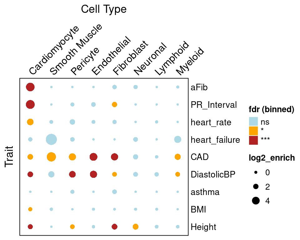
| Version | Author | Date |
|---|---|---|
| 39e9a66 | kevinlkx | 2022-04-19 |
sessionInfo()R version 4.2.0 (2022-04-22)
Platform: x86_64-pc-linux-gnu (64-bit)
Running under: CentOS Linux 7 (Core)
Matrix products: default
BLAS/LAPACK: /software/openblas-0.3.13-el7-x86_64/lib/libopenblas_haswellp-r0.3.13.so
locale:
[1] LC_CTYPE=en_US.UTF-8 LC_NUMERIC=C LC_TIME=C
[4] LC_COLLATE=C LC_MONETARY=C LC_MESSAGES=C
[7] LC_PAPER=C LC_NAME=C LC_ADDRESS=C
[10] LC_TELEPHONE=C LC_MEASUREMENT=C LC_IDENTIFICATION=C
attached base packages:
[1] grid stats4 stats graphics grDevices utils datasets
[8] methods base
other attached packages:
[1] ComplexHeatmap_2.12.0
[2] liftOver_1.20.0
[3] Homo.sapiens_1.3.1
[4] TxDb.Hsapiens.UCSC.hg19.knownGene_3.2.2
[5] org.Hs.eg.db_3.15.0
[6] GO.db_3.15.0
[7] OrganismDbi_1.38.1
[8] GenomicFeatures_1.50.4
[9] AnnotationDbi_1.60.0
[10] Biobase_2.58.0
[11] rtracklayer_1.58.0
[12] GenomicRanges_1.48.0
[13] GenomeInfoDb_1.34.9
[14] IRanges_2.32.0
[15] S4Vectors_0.36.1
[16] BiocGenerics_0.44.0
[17] gwascat_2.28.1
[18] forcats_1.0.0
[19] stringr_1.5.0
[20] dplyr_1.1.0
[21] purrr_1.0.1
[22] readr_2.1.4
[23] tidyr_1.3.0
[24] tibble_3.1.8
[25] ggplot2_3.4.1
[26] tidyverse_1.3.2
[27] mapgen_0.5.6
[28] workflowr_1.7.0
loaded via a namespace (and not attached):
[1] circlize_0.4.15 readxl_1.4.2
[3] backports_1.4.1 BiocFileCache_2.6.0
[5] splines_4.2.0 BiocParallel_1.32.5
[7] digest_0.6.31 foreach_1.5.2
[9] htmltools_0.5.4 fansi_1.0.4
[11] magrittr_2.0.3 memoise_2.0.1
[13] BSgenome_1.66.2 cluster_2.1.3
[15] doParallel_1.0.17 googlesheets4_1.0.1
[17] tzdb_0.3.0 Biostrings_2.66.0
[19] modelr_0.1.10 matrixStats_0.63.0
[21] timechange_0.2.0 prettyunits_1.1.1
[23] colorspace_2.1-0 blob_1.2.3
[25] rvest_1.0.3 rappdirs_0.3.3
[27] haven_2.5.1 xfun_0.37
[29] callr_3.7.3 crayon_1.5.2
[31] RCurl_1.98-1.10 jsonlite_1.8.4
[33] graph_1.74.0 iterators_1.0.14
[35] survival_3.3-1 VariantAnnotation_1.44.1
[37] glue_1.6.2 gtable_0.3.1
[39] gargle_1.3.0 zlibbioc_1.44.0
[41] XVector_0.38.0 GetoptLong_1.0.5
[43] DelayedArray_0.24.0 shape_1.4.6
[45] scales_1.2.1 DBI_1.1.3
[47] Rcpp_1.0.10 progress_1.2.2
[49] clue_0.3-61 bit_4.0.5
[51] httr_1.4.4 RColorBrewer_1.1-3
[53] ellipsis_0.3.2 pkgconfig_2.0.3
[55] XML_3.99-0.13 sass_0.4.5
[57] dbplyr_2.3.0 utf8_1.2.3
[59] tidyselect_1.2.0 rlang_1.0.6
[61] later_1.3.0 munsell_0.5.0
[63] cellranger_1.1.0 tools_4.2.0
[65] cachem_1.0.6 cli_3.6.0
[67] generics_0.1.3 RSQLite_2.2.20
[69] broom_1.0.3 evaluate_0.20
[71] fastmap_1.1.0 yaml_2.3.7
[73] processx_3.8.0 knitr_1.42
[75] bit64_4.0.5 fs_1.6.1
[77] KEGGREST_1.38.0 RBGL_1.72.0
[79] whisker_0.4 xml2_1.3.3
[81] biomaRt_2.54.0 compiler_4.2.0
[83] rstudioapi_0.14 filelock_1.0.2
[85] curl_5.0.0 png_0.1-8
[87] reprex_2.0.2 bslib_0.4.2
[89] stringi_1.7.12 highr_0.10
[91] ps_1.7.2 lattice_0.20-45
[93] Matrix_1.5-3 vctrs_0.5.2
[95] pillar_1.8.1 lifecycle_1.0.3
[97] BiocManager_1.30.18 GlobalOptions_0.1.2
[99] jquerylib_0.1.4 snpStats_1.46.0
[101] bitops_1.0-7 httpuv_1.6.5
[103] R6_2.5.1 BiocIO_1.8.0
[105] promises_1.2.0.1 codetools_0.2-18
[107] assertthat_0.2.1 SummarizedExperiment_1.28.0
[109] rprojroot_2.0.3 rjson_0.2.21
[111] withr_2.5.0 GenomicAlignments_1.34.0
[113] Rsamtools_2.12.0 GenomeInfoDbData_1.2.9
[115] parallel_4.2.0 hms_1.1.2
[117] rmarkdown_2.20 MatrixGenerics_1.10.0
[119] googledrive_2.0.0 Cairo_1.6-0
[121] git2r_0.30.1 getPass_0.2-2
[123] lubridate_1.9.2 restfulr_0.0.15