Unguided GSFA analysis on LUHMES CROP-seq data

workflowr

• Summary
• Checks
• Past versions

Last updated: 2022-09-20

Checks: 7 0

Knit directory: GSFA_analysis/

This reproducible R Markdown analysis was created with workflowr (version 1.7.0). The Checks tab describes the reproducibility checks that were applied when the results were created. The Past versions tab lists the development history.

---

R Markdown file: up-to-date

Great! Since the R Markdown file has been committed to the Git repository, you know the exact version of the code that produced these results.

Environment: empty

Great job! The global environment was empty. Objects defined in the global environment can affect the analysis in your R Markdown file in unknown ways. For reproduciblity it’s best to always run the code in an empty environment.

Seed: set.seed(20220524)

The command set.seed(20220524) was run prior to running the code in the R Markdown file. Setting a seed ensures that any results that rely on randomness, e.g. subsampling or permutations, are reproducible.

Session information: recorded

Great job! Recording the operating system, R version, and package versions is critical for reproducibility.

Cache: none

Nice! There were no cached chunks for this analysis, so you can be confident that you successfully produced the results during this run.

File paths: relative

Great job! Using relative paths to the files within your workflowr project makes it easier to run your code on other machines.

Repository version: d23cb3c

Great! You are using Git for version control. Tracking code development and connecting the code version to the results is critical for reproducibility.

The results in this page were generated with repository version d23cb3c. See the Past versions tab to see a history of the changes made to the R Markdown and HTML files.

Note that you need to be careful to ensure that all relevant files for the analysis have been committed to Git prior to generating the results (you can use wflow_publish or wflow_git_commit). workflowr only checks the R Markdown file, but you know if there are other scripts or data files that it depends on. Below is the status of the Git repository when the results were generated:

Ignored files:
    Ignored:    .DS_Store
    Ignored:    .Rhistory
    Ignored:    .Rproj.user/

Untracked files:
    Untracked:  Rplots.pdf
    Untracked:  analysis/check_Tcells_datasets.Rmd
    Untracked:  analysis/fscLVM_analysis.Rmd
    Untracked:  analysis/spca_LUHMES_data.Rmd
    Untracked:  analysis/test_seurat.Rmd
    Untracked:  code/gsfa_negctrl_job.sbatch
    Untracked:  code/music_LUHMES_Yifan.R
    Untracked:  code/plotting_functions.R
    Untracked:  code/run_fscLVM_LUHMES_data.R
    Untracked:  code/run_gsfa_2groups_negctrl.R
    Untracked:  code/run_gsfa_negctrl.R
    Untracked:  code/run_music_LUHMES.R
    Untracked:  code/run_music_LUHMES_data.sbatch
    Untracked:  code/run_music_LUHMES_data_20topics.R
    Untracked:  code/run_music_LUHMES_data_20topics.sbatch
    Untracked:  code/run_sceptre_Tcells_data.sbatch
    Untracked:  code/run_sceptre_Tcells_stimulated_data.sbatch
    Untracked:  code/run_sceptre_Tcells_test_data.sbatch
    Untracked:  code/run_sceptre_Tcells_unstimulated_data.sbatch
    Untracked:  code/run_sceptre_permuted_data.sbatch
    Untracked:  code/run_spca_LUHMES.R
    Untracked:  code/run_spca_TCells.R
    Untracked:  code/run_twostep_clustering_LUHMES_data.sbatch
    Untracked:  code/run_twostep_clustering_Tcells_data.sbatch
    Untracked:  code/run_unguided_gsfa_LUHMES.R
    Untracked:  code/run_unguided_gsfa_LUHMES.sbatch
    Untracked:  code/run_unguided_gsfa_Tcells.R
    Untracked:  code/run_unguided_gsfa_Tcells.sbatch
    Untracked:  code/sceptre_LUHMES_data.R
    Untracked:  code/sceptre_Tcells_stimulated_data.R
    Untracked:  code/sceptre_Tcells_unstimulated_data.R
    Untracked:  code/sceptre_permutation_analysis.R
    Untracked:  code/sceptre_permute_analysis.R
    Untracked:  code/seurat_sim_fpr_tpr.R
    Untracked:  code/unguided_GFSA_mixture_normal_prior.cpp

Unstaged changes:
    Modified:   analysis/sceptre_TCells_data.Rmd
    Modified:   code/run_sceptre_LUHMES_data.R
    Modified:   code/run_sceptre_LUHMES_data.sbatch
    Modified:   code/run_sceptre_LUHMES_permuted_data.R
    Modified:   code/run_sceptre_Tcells_permuted_data.R
    Modified:   code/run_sceptre_cropseq_data.sbatch
    Modified:   code/run_twostep_clustering_LUHMES_data.R
    Modified:   code/sceptre_analysis.R

Note that any generated files, e.g. HTML, png, CSS, etc., are not included in this status report because it is ok for generated content to have uncommitted changes.

---

These are the previous versions of the repository in which changes were made to the R Markdown (analysis/unguided_gsfa_LUHMES_data.Rmd) and HTML (docs/unguided_gsfa_LUHMES_data.html) files. If you’ve configured a remote Git repository (see ?wflow_git_remote), click on the hyperlinks in the table below to view the files as they were in that past version.

File	Version	Author	Date	Message
Rmd	d23cb3c	kevinlkx	2022-09-20	updated the size of qq plots
html	3691834	kevinlkx	2022-09-03	Build site.
Rmd	6dea756	kevinlkx	2022-09-03	updated qq plots
html	04eadb5	kevinlkx	2022-09-01	Build site.
Rmd	659804b	kevinlkx	2022-09-01	updated QQplot colors
html	472cbfa	kevinlkx	2022-09-01	Build site.
Rmd	4834f30	kevinlkx	2022-09-01	added QQ plot for GSFA vs MAST
html	e70e2ab	kevinlkx	2022-08-31	Build site.
Rmd	04f09bd	kevinlkx	2022-08-31	added qqplots for combined results
html	8b0d5f1	kevinlkx	2022-08-25	Build site.
Rmd	d98fea7	kevinlkx	2022-08-25	plot betas in the dotplots
html	51fd61a	kevinlkx	2022-08-25	Build site.
Rmd	7b115b5	kevinlkx	2022-08-25	unguided GSFA res for LUHMES data
html	a561ed8	kevinlkx	2022-08-25	Build site.
Rmd	150dbc1	kevinlkx	2022-08-25	unguided GSFA res for LUHMES data
html	2cefbda	kevinlkx	2022-08-25	Build site.
Rmd	ae5b1ad	kevinlkx	2022-08-25	unguided GSFA res for LUHMES data

---

mkdir -p /project2/xinhe/kevinluo/GSFA/data

cp /project2/xinhe/yifan/Factor_analysis/LUHMES/processed_data/deviance_residual.merged_top_6k.corrected_4.scaled.rds \
  /project2/xinhe/kevinluo/GSFA/unguided_GSFA/LUHMES/processed_data/deviance_residual.merged_top_6k.corrected_4.scaled.rds

cp /project2/xinhe/yifan/Factor_analysis/LUHMES/processed_data/merged_metadata.rds \
  /project2/xinhe/kevinluo/GSFA/unguided_GSFA/LUHMES/processed_data/merged_metadata.rds

Analysis scripts

• R script: /home/kaixuan/projects/GSFA_analysis/code/run_unguided_gsfa_LUHMES.R
  
• sbatch script: /home/kaixuan/projects/GSFA_analysis/code/run_unguided_gsfa_LUHMES.sbatch

mkdir -p /project2/xinhe/kevinluo/GSFA/unguided_GSFA/log
cd /project2/xinhe/kevinluo/GSFA/unguided_GSFA/log

sbatch ~/projects/GSFA_analysis/code/run_unguided_gsfa_LUHMES.sbatch

Load packages

suppressPackageStartupMessages(library(data.table))
# suppressPackageStartupMessages(library(Seurat))
suppressPackageStartupMessages(library(ComplexHeatmap))
suppressPackageStartupMessages(library(ggplot2))
require(reshape2)
require(dplyr)
require(ComplexHeatmap)
theme_set(theme_bw() + theme(plot.title = element_text(size = 14, hjust = 0.5),
                             axis.title = element_text(size = 14),
                             axis.text = element_text(size = 13),
                             legend.title = element_text(size = 13),
                             legend.text = element_text(size = 12),
                             panel.grid.minor = element_blank())
)
suppressPackageStartupMessages(library(gridExtra))
source("code/plotting_functions.R")

Set directories

res_dir <- "/project2/xinhe/kevinluo/GSFA/unguided_GSFA/LUHMES/"
dir.create(res_dir, recursive = TRUE, showWarnings = FALSE)

Load unguided GSFA result

fit <- readRDS("/project2/xinhe/kevinluo/GSFA/unguided_GSFA/LUHMES/unguided_gsfa_output/All.gibbs_obj_k20.unguided.svd.seed_14314.light.rds")

Load the cell by perturbation matrix.

data_folder <- "/project2/xinhe/kevinluo/GSFA/unguided_GSFA/LUHMES/"
metadata <- readRDS(paste0(data_folder, "processed_data/merged_metadata.rds"))
# Perturbation info:
G_mat <- metadata[, 4:18]
G_mat <- as.matrix(G_mat)
KO_names <- colnames(G_mat)
negctrl_index <- which(KO_names == "Nontargeting")

Use linear regression to test for the association between perturbations and factors

Z_pm <- fit$posterior_means$Z_pm
if(!all.equal(rownames(G_mat), rownames(Z_pm))){
  stop("Rownames of G_mat do not match with Z_pm!")
}

perturb_matrix <- G_mat
factor_matrix <- Z_pm

summary_df <- expand.grid(colnames(perturb_matrix), colnames(factor_matrix))
colnames(summary_df) <- c("perturb", "factor")

summary_df <- cbind(summary_df, beta = NA, statistic = NA, pval = NA)

for(i in 1:nrow(summary_df)){
  df <- data.frame(perturb = perturb_matrix[,summary_df$perturb[i]], 
                   factor = factor_matrix[,summary_df$factor[i]])
  lm.res <- lm(factor ~ perturb, data=df)
  summary_df[i, ]$beta <- summary(lm.res)$coefficients["perturb",1]
  summary_df[i, ]$statistic <- summary(lm.res)$coefficients["perturb",3]
  summary_df[i, ]$pval <- summary(lm.res)$coefficients["perturb",4]
}

summary_df$fdr <- p.adjust(summary_df$pval, method = "BH")
summary_df$bonferroni_adj <- p.adjust(summary_df$pval, method = "bonferroni")

saveRDS(summary_df, file = file.path(res_dir, "LUHMES_unguidedGSFA_guide_factor_lm_summary_df.rds"))

stat_mat <- reshape2::dcast(summary_df %>% dplyr::select(perturb, factor, statistic), perturb ~ factor, value.var = "statistic") 
rownames(stat_mat) <- stat_mat$perturb
stat_mat$perturb <- NULL
stat_mat <- as.matrix(stat_mat)

beta_mat <- reshape2::dcast(summary_df %>% dplyr::select(perturb, factor, beta), perturb ~ factor, value.var = "beta")
rownames(beta_mat) <- beta_mat$perturb
beta_mat$perturb <- NULL
beta_mat <- as.matrix(beta_mat)

fdr_mat <- reshape2::dcast(summary_df %>% dplyr::select(perturb, factor, fdr), perturb ~ factor, value.var = "fdr")
rownames(fdr_mat) <- fdr_mat$perturb
fdr_mat$perturb <- NULL
fdr_mat <- as.matrix(fdr_mat)

bonferroni_mat <- reshape2::dcast(summary_df %>% dplyr::select(perturb, factor, bonferroni_adj), 
                                  perturb ~ factor, value.var = "bonferroni_adj")
rownames(bonferroni_mat) <- bonferroni_mat$perturb
bonferroni_mat$perturb <- NULL
bonferroni_mat <- as.matrix(bonferroni_mat)

# pdf(file.path(res_dir, "stat-fdr-dotplot.pdf"), width = 9, height = 5.5)
KO_names <- rownames(fdr_mat)
dotplot_effectsize(t(beta_mat), t(fdr_mat),
                   reorder_markers = c(KO_names[KO_names!="Nontargeting"], "Nontargeting"),
                   color_lgd_title = "Estimated effect size",
                   size_lgd_title = "FDR",
                   max_score = 0.6,
                   min_score = -0.6,
                   by_score = 0.3) + coord_flip()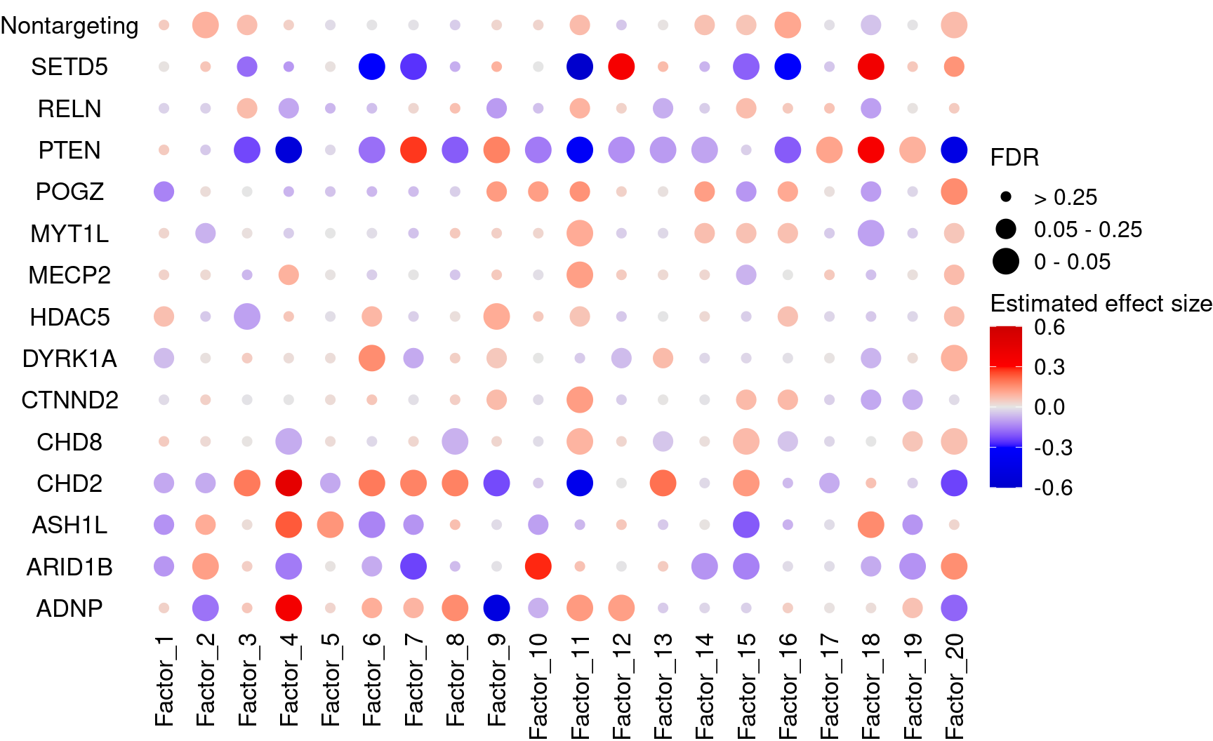

Past versions of stat-fdr-dotplot-1.png

Version	Author	Date
8b0d5f1	kevinlkx	2022-08-25
2cefbda	kevinlkx	2022-08-25

# dev.off()

Plot perturbation ~ cluster associations (show Bonferroni adjusted p-values)

# pdf(file.path(res_dir, "stat-bonferroni-dotplot.pdf"), width = 9, height = 5.5)
KO_names <- rownames(bonferroni_mat)
dotplot_effectsize(t(beta_mat), t(bonferroni_mat),
                   reorder_markers = c(KO_names[KO_names!="Nontargeting"], "Nontargeting"),
                   color_lgd_title = "Estimated effect size",
                   size_lgd_title = "Bonferroni\nadjusted p-value",
                   max_score = 0.6,
                   min_score = -0.6,
                   by_score = 0.3) + coord_flip()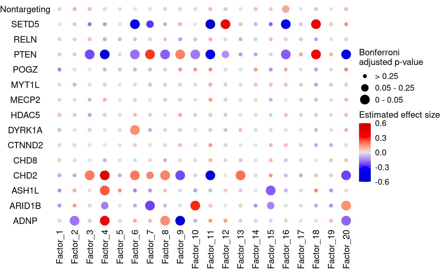

Past versions of stat-bonferroni-dotplot-1.png

Version	Author	Date
8b0d5f1	kevinlkx	2022-08-25
2cefbda	kevinlkx	2022-08-25

# dev.off()

Find DE genes for each factor and assign DE genes to associated perturbations

First, find DE genes for each factor using F matrix (PIP>0.95).

Then, for each perturbation, find the associated factors, and pull the DE genes for those factors.

F_pm <- fit$posterior_means$F_pm
# dim(F_pm)
# feature.names <- data.frame(fread(file.path(data_dir, "LUHMES_GSM4219575_Run1_genes.tsv.gz"),
#                                   header = FALSE), stringsAsFactors = FALSE)

de.genes.factors <- vector("list", length = ncol(F_pm))
names(de.genes.factors) <- colnames(F_pm)
for( i in 1:length(de.genes.factors)){
  de_genes <- rownames(F_pm[F_pm[,i] > 0.95,])
  # de_genes <- feature.names$V2[match(de_genes, feature.names$V1)]
  de.genes.factors[[i]] <- de_genes
}

Number of DE genes for each perturbation (FDR < 0.05)

perturb_names <- colnames(perturb_matrix)
perturb_names <- c("Nontargeting", perturb_names[perturb_names!="Nontargeting"])

de.genes.perturbs <- vector("list", length = length(perturb_names))
names(de.genes.perturbs) <- perturb_names

for(i in 1:length(de.genes.perturbs)){
  perturb_name <- names(de.genes.perturbs)[i]
  associated_factors <- colnames(fdr_mat)[which(fdr_mat[perturb_name, ] < 0.05)]
  if(length(associated_factors) > 0){
    de.genes.perturbs[[i]] <- unique(unlist(de.genes.factors[associated_factors]))
  }
}

num.de.genes.perturbs <- sapply(de.genes.perturbs, length)

unguided_GSFA_fdr0.05_genes <- de.genes.perturbs

dge_plot_df <- data.frame(Perturbation = names(num.de.genes.perturbs), Num_DEGs = num.de.genes.perturbs)
dge_plot_df$Perturbation <- factor(dge_plot_df$Perturbation, levels = names(num.de.genes.perturbs))

# pdf(file.path(res_dir, "count-de-genes.pdf"), width = 13, height = 5)
ggplot(data=dge_plot_df, aes(x = Perturbation, y = Num_DEGs+1)) +
  geom_bar(position = "dodge", stat = "identity") +
  geom_text(aes(label = Num_DEGs), position=position_dodge(width=0.9), vjust=-0.25) +
  scale_y_log10() +
  scale_fill_brewer(palette = "Set2") +
  labs(x = "Target gene",
       y = "Number of DEGs",
       title = "Number of DEGs detected by unguided GSFA") +
  theme(axis.text.x = element_text(angle = 45, hjust = 1, size = 12),
        legend.position = "bottom",
        legend.text = element_text(size = 13))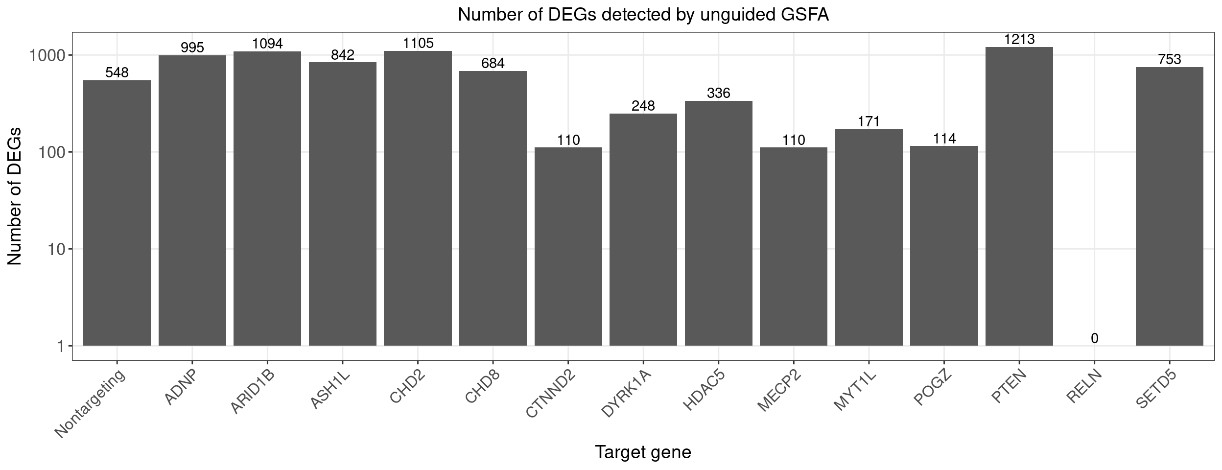

Past versions of count-de-genes-fdr-1.png

Version	Author	Date
2cefbda	kevinlkx	2022-08-25

# dev.off()

Number of DE genes for each perturbation (Bonferroni adjusted p-value < 0.05)

perturb_names <- colnames(perturb_matrix)
perturb_names <- c("Nontargeting", perturb_names[perturb_names!="Nontargeting"])

de.genes.perturbs <- vector("list", length = length(perturb_names))
names(de.genes.perturbs) <- perturb_names

for(i in 1:length(de.genes.perturbs)){
  perturb_name <- names(de.genes.perturbs)[i]
  associated_factors <- colnames(bonferroni_mat)[which(bonferroni_mat[perturb_name, ] < 0.05)]
  if(length(associated_factors) > 0){
    de.genes.perturbs[[i]] <- unique(unlist(de.genes.factors[associated_factors]))
  }
}

num.de.genes.perturbs <- sapply(de.genes.perturbs, length)
unguided_GSFA_bonferroni0.05_genes <- de.genes.perturbs

dge_plot_df <- data.frame(Perturbation = names(num.de.genes.perturbs), Num_DEGs = num.de.genes.perturbs)
dge_plot_df$Perturbation <- factor(dge_plot_df$Perturbation, levels = names(num.de.genes.perturbs))

ggplot(data=dge_plot_df, aes(x = Perturbation, y = Num_DEGs+1)) +
  geom_bar(position = "dodge", stat = "identity") +
  geom_text(aes(label = Num_DEGs), position=position_dodge(width=0.9), vjust=-0.25) +
  scale_y_log10() +
  scale_fill_brewer(palette = "Set2") +
  labs(x = "Target gene",
       y = "Number of DEGs",
       title = "Number of DEGs detected by unguided GSFA") +
  theme(axis.text.x = element_text(angle = 45, hjust = 1, size = 12),
        legend.position = "bottom",
        legend.text = element_text(size = 13))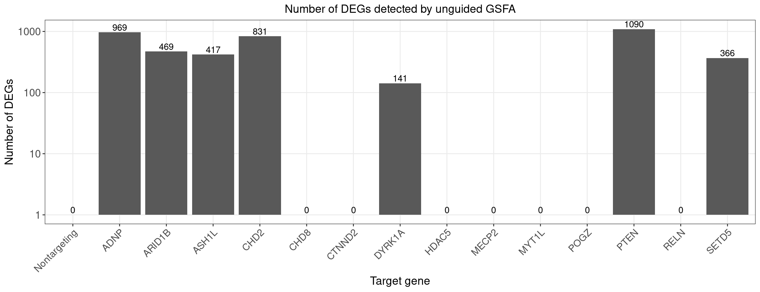

Past versions of count-de-genes-bonferroni-1.png

Version	Author	Date
2cefbda	kevinlkx	2022-08-25

Compare single-gene DE p-value distributions between GSFA and unguided GSFA

fdr_cutoff <- 0.05
lfsr_cutoff <- 0.05

Load the output of GSFA fit_gsfa_multivar() run.

data_folder <- "/project2/xinhe/yifan/Factor_analysis/LUHMES/"
fit <- readRDS(paste0(data_folder,
                      "gsfa_output_detect_01/use_negctrl/All.gibbs_obj_k20.svd_negctrl.seed_14314.light.rds"))
gibbs_PM <- fit$posterior_means
lfsr_mat <- fit$lfsr[, -ncol(fit$lfsr)]
total_effect <- fit$total_effect[, -ncol(fit$total_effect)]
KO_names <- colnames(lfsr_mat)

DEGs detected by GSFA

        ADNP       ARID1B        ASH1L         CHD2         CHD8       CTNND2 
         795          310          322          756            0            0 
      DYRK1A        HDAC5        MECP2        MYT1L Nontargeting         POGZ 
          23            0            0            0            0            0 
        PTEN         RELN        SETD5 
         895            0          466 

Load MAST single-gene DE result

guides <- KO_names[KO_names!="Nontargeting"]

mast_list <- list()
for (m in guides){
  fname <- paste0(data_folder, "processed_data/MAST/dev_top6k_negctrl/gRNA_", m, ".dev_res_top6k.vs_negctrl.rds")
  tmp_df <- readRDS(fname)
  tmp_df$geneID <- rownames(tmp_df)
  tmp_df <- tmp_df %>% dplyr::rename(FDR = fdr, PValue = pval)
  mast_list[[m]] <- tmp_df
}
mast_signif_counts <- sapply(mast_list, function(x){filter(x, FDR < fdr_cutoff) %>% nrow()})
# summary(mast_list)

QQ-plots of MAST DE p-values for the GSFA genes vs unguided GSFA genes.

qqplots <- list()
for(i in 1:length(guides)){
  guide <- guides[i]
  mast_res <- mast_list[[guide]]
  unguided_gsfa_de_genes <- unguided_GSFA_fdr0.05_genes[[guide]]
  gsfa_de_genes <- gsfa_sig_genes[[guide]]
  unguided_gsfa_de_genes <- intersect(unguided_gsfa_de_genes, rownames(mast_res))
  gsfa_de_genes <- intersect(gsfa_de_genes, rownames(mast_res))
  
  if(length(unguided_gsfa_de_genes)>0 && length(gsfa_de_genes) >0){
    mast_res$unguided_gsfa_gene <- 0
    mast_res[unguided_gsfa_de_genes, ]$unguided_gsfa_gene <- 1
    mast_res$gsfa_gene <- 0
    mast_res[gsfa_de_genes, ]$gsfa_gene <- 1
    pvalue_list <- list('Unguided GSFA'=dplyr::filter(mast_res,unguided_gsfa_gene==1)$PValue,
                        'GSFA'=dplyr::filter(mast_res,gsfa_gene==1)$PValue,
                        'all genes'=mast_res$PValue)
    qqplots[[guide]] <- qqplot.pvalue(pvalue_list, pointSize = 1, legendSize = 4) + 
      ggtitle(guide) + theme(plot.title = element_text(hjust = 0.5))
  }
}

grid.arrange(grobs = qqplots, nrow = 4, ncol = 2)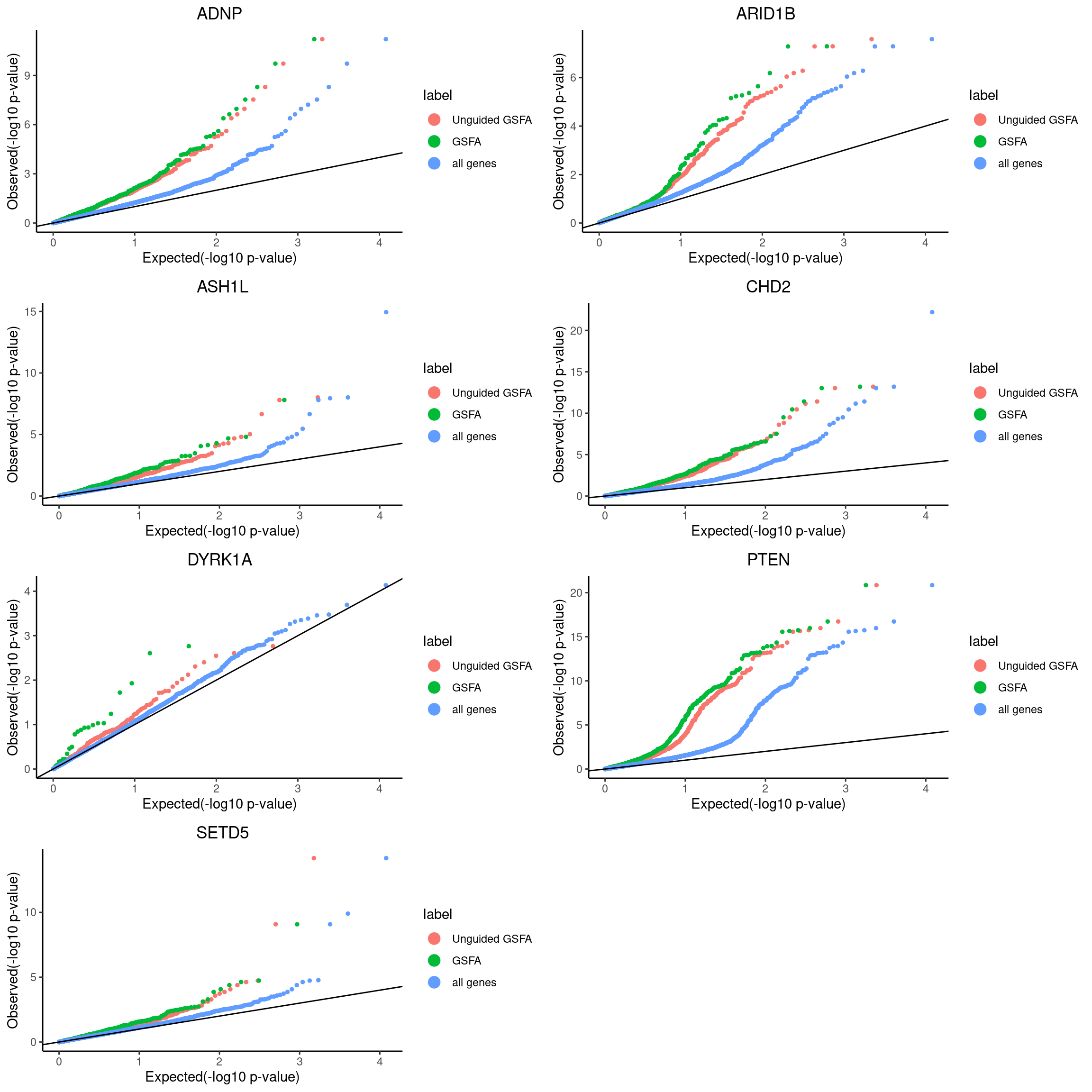

Past versions of qqplots-gsfa-unguided-all-1.png

Version	Author	Date
3691834	kevinlkx	2022-09-03
2cefbda	kevinlkx	2022-08-25

Pooling p-values from all perturbations

combined_mast_res <- data.frame()
for(i in 1:length(guides)){
  guide <- guides[i]
  mast_res <- mast_list[[guide]]
  unguided_gsfa_de_genes <- unguided_GSFA_fdr0.05_genes[[guide]]
  gsfa_de_genes <- gsfa_sig_genes[[guide]]
  unguided_gsfa_de_genes <- intersect(unguided_gsfa_de_genes, rownames(mast_res))
  gsfa_de_genes <- intersect(gsfa_de_genes, rownames(mast_res))
  mast_res$unguided_gsfa_gene <- 0
  if(length(unguided_gsfa_de_genes) >0){
    mast_res[unguided_gsfa_de_genes, ]$unguided_gsfa_gene <- 1
  }
  mast_res$gsfa_gene <- 0
  if(length(gsfa_de_genes) >0){
    mast_res[gsfa_de_genes, ]$gsfa_gene <- 1
  }
  combined_mast_res <- rbind(combined_mast_res, mast_res)
}

pvalue_list <- list('Unguided GSFA'=dplyr::filter(combined_mast_res,unguided_gsfa_gene==1)$PValue,
                    'GSFA'=dplyr::filter(combined_mast_res,gsfa_gene==1)$PValue,
                    'all genes'=combined_mast_res$PValue)

# pdf(file.path(res_dir, "qqplot_all_combined.pdf"))
qqplot.pvalue(pvalue_list, pointSize = 1, legendSize = 4) + 
      ggtitle("") + theme(plot.title = element_text(hjust = 0.5)) +
      scale_colour_discrete(name="Method")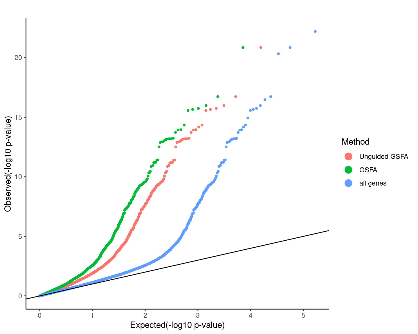

Past versions of qqplots-gsfa-unguided-all-combined-1.png

Version	Author	Date
3691834	kevinlkx	2022-09-03
e70e2ab	kevinlkx	2022-08-31

# dev.off()

QQ-plots of MAST DE p-values for the GSFA only genes vs two-step only genes.

qqplots <- list()
for(i in 1:length(guides)){
  guide <- guides[i]
  mast_res <- mast_list[[guide]]
  unguided_gsfa_de_genes <- unguided_GSFA_fdr0.05_genes[[guide]]
  gsfa_de_genes <- gsfa_sig_genes[[guide]]
  unguided_gsfa_de_genes <- intersect(unguided_gsfa_de_genes, rownames(mast_res))
  gsfa_de_genes <- intersect(gsfa_de_genes, rownames(mast_res))
  
  if(length(unguided_gsfa_de_genes)>0 && length(gsfa_de_genes) >0){
    mast_res$unguided_gsfa_only_gene <- 0
    mast_res[setdiff(unguided_gsfa_de_genes, gsfa_de_genes), ]$unguided_gsfa_only_gene <- 1
    mast_res$gsfa_only_gene <- 0
    mast_res[setdiff(gsfa_de_genes, unguided_gsfa_de_genes), ]$gsfa_only_gene <- 1
    
    pvalue_list <- list('Unguided GSFA only'=dplyr::filter(mast_res,unguided_gsfa_only_gene==1)$PValue,
                        'GSFA only'=dplyr::filter(mast_res,gsfa_only_gene==1)$PValue,
                        'all genes'=mast_res$PValue)
    qqplots[[guide]] <- qqplot.pvalue(pvalue_list, pointSize = 1, legendSize = 4) + 
      ggtitle(guide) + theme(plot.title = element_text(hjust = 0.5))
  }
}

grid.arrange(grobs = qqplots, nrow = 4, ncol = 2)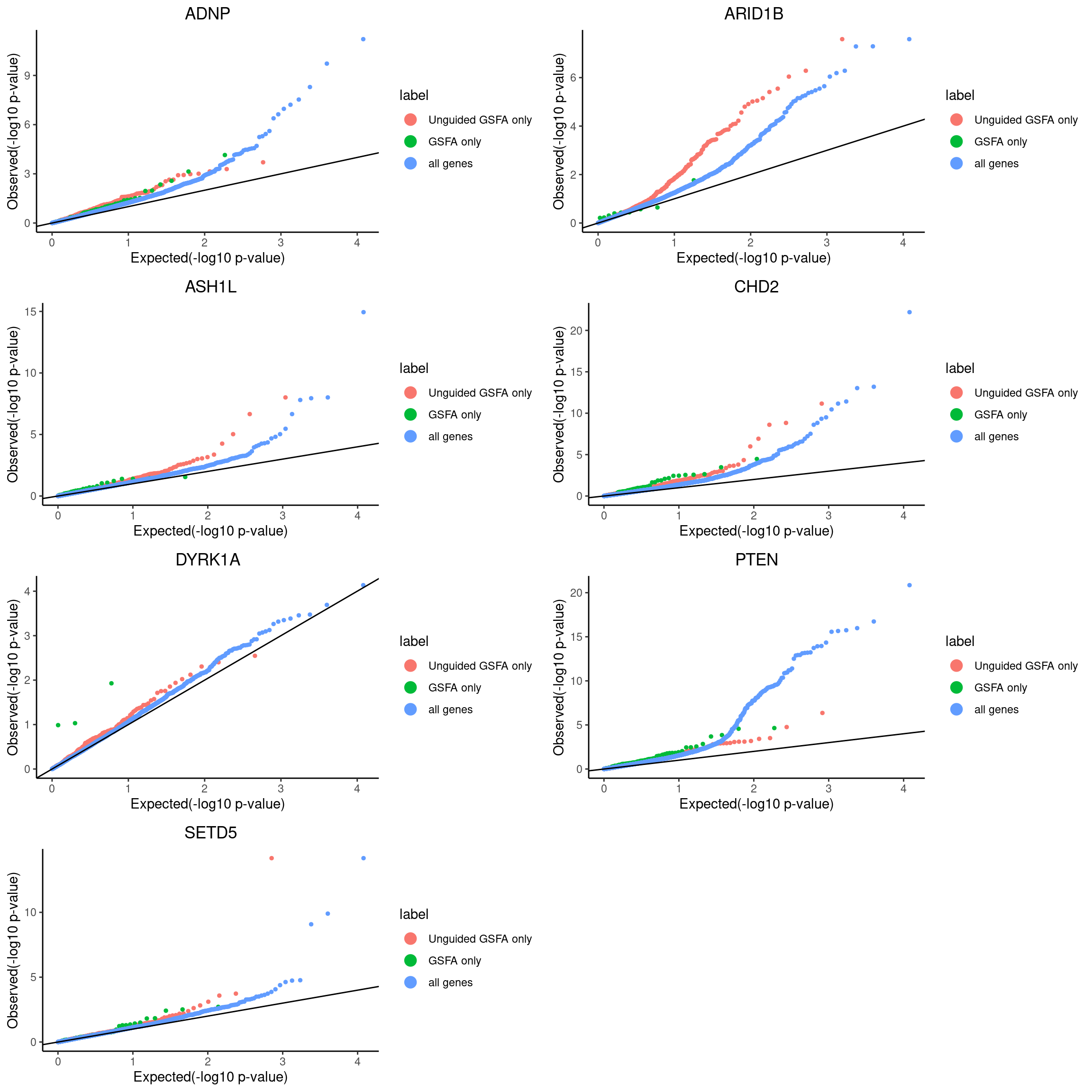

Past versions of qqplots-gsfa-unguided-only-1.png

Version	Author	Date
3691834	kevinlkx	2022-09-03
2cefbda	kevinlkx	2022-08-25

Pooling p-values from all perturbations

combined_mast_res <- data.frame()
for(i in 1:length(guides)){
  guide <- guides[i]
  mast_res <- mast_list[[guide]]
  unguided_gsfa_de_genes <- unguided_GSFA_fdr0.05_genes[[guide]]
  gsfa_de_genes <- gsfa_sig_genes[[guide]]
  unguided_gsfa_de_genes <- intersect(unguided_gsfa_de_genes, rownames(mast_res))
  gsfa_de_genes <- intersect(gsfa_de_genes, rownames(mast_res))
  mast_res$unguided_gsfa_only_gene <- 0
  if(length(setdiff(unguided_gsfa_de_genes, gsfa_de_genes)) >0){
    mast_res[setdiff(unguided_gsfa_de_genes, gsfa_de_genes), ]$unguided_gsfa_only_gene <- 1
  }
  mast_res$gsfa_only_gene <- 0
  if(length(setdiff(gsfa_de_genes, unguided_gsfa_de_genes)) >0){
    mast_res[setdiff(gsfa_de_genes, unguided_gsfa_de_genes), ]$gsfa_only_gene <- 1
  }
  combined_mast_res <- rbind(combined_mast_res, mast_res)
}

pvalue_list <- list('Unguided GSFA only'=dplyr::filter(combined_mast_res,unguided_gsfa_only_gene==1)$PValue,
                    'GSFA only'=dplyr::filter(combined_mast_res,gsfa_only_gene==1)$PValue,
                    'all genes'=combined_mast_res$PValue)

# pdf(file.path(res_dir, "qqplot_only_combined.pdf"))
qqplot.pvalue(pvalue_list, pointSize = 1, legendSize = 4) + 
      ggtitle("") + theme(plot.title = element_text(hjust = 0.5)) +
      scale_colour_discrete(name="Method")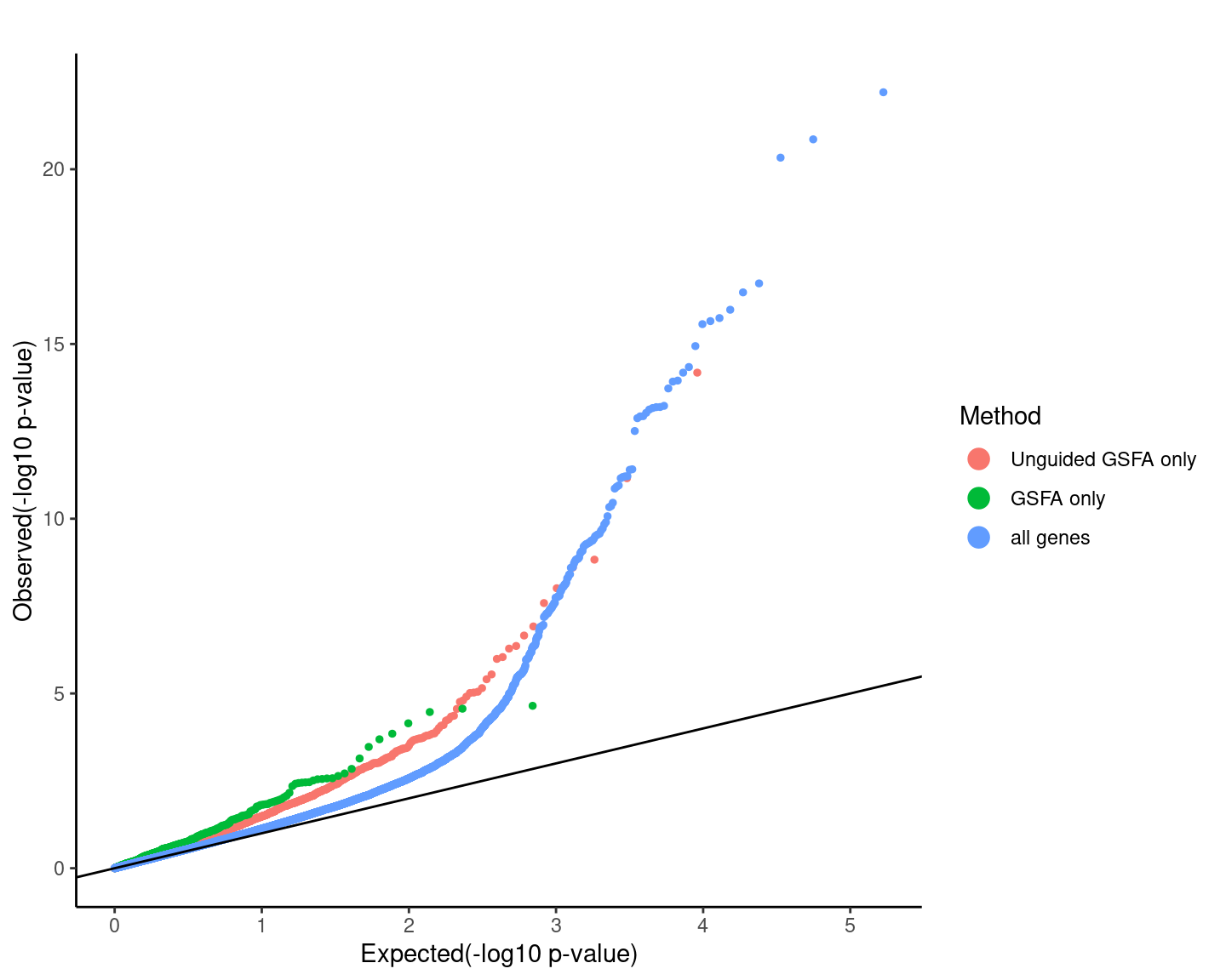

Past versions of qqplots-gsfa-unguided-only-combined-1.png

Version	Author	Date
3691834	kevinlkx	2022-09-03
e70e2ab	kevinlkx	2022-08-31

# dev.off()

Session information

sessionInfo()

R version 4.2.0 (2022-04-22)
Platform: x86_64-pc-linux-gnu (64-bit)
Running under: CentOS Linux 7 (Core)

Matrix products: default
BLAS/LAPACK: /software/openblas-0.3.13-el7-x86_64/lib/libopenblas_haswellp-r0.3.13.so

locale:
 [1] LC_CTYPE=en_US.UTF-8 LC_NUMERIC=C         LC_TIME=C           
 [4] LC_COLLATE=C         LC_MONETARY=C        LC_MESSAGES=C       
 [7] LC_PAPER=C           LC_NAME=C            LC_ADDRESS=C        
[10] LC_TELEPHONE=C       LC_MEASUREMENT=C     LC_IDENTIFICATION=C 

attached base packages:
[1] grid      stats     graphics  grDevices utils     datasets  methods  
[8] base     

other attached packages:
[1] lattice_0.20-45       gridExtra_2.3         dplyr_1.0.9          
[4] reshape2_1.4.4        ggplot2_3.3.6         ComplexHeatmap_2.12.0
[7] data.table_1.14.2     workflowr_1.7.0      

loaded via a namespace (and not attached):
 [1] Rcpp_1.0.8.3        circlize_0.4.15     getPass_0.2-2      
 [4] png_0.1-7           ps_1.7.0            assertthat_0.2.1   
 [7] rprojroot_2.0.3     digest_0.6.29       foreach_1.5.2      
[10] utf8_1.2.2          plyr_1.8.7          R6_2.5.1           
[13] stats4_4.2.0        evaluate_0.15       highr_0.9          
[16] httr_1.4.3          pillar_1.7.0        GlobalOptions_0.1.2
[19] rlang_1.0.2         rstudioapi_0.13     whisker_0.4        
[22] callr_3.7.0         jquerylib_0.1.4     S4Vectors_0.34.0   
[25] GetoptLong_1.0.5    rmarkdown_2.14      labeling_0.4.2     
[28] stringr_1.4.0       munsell_0.5.0       compiler_4.2.0     
[31] httpuv_1.6.5        xfun_0.30           pkgconfig_2.0.3    
[34] BiocGenerics_0.42.0 shape_1.4.6         htmltools_0.5.2    
[37] tidyselect_1.1.2    tibble_3.1.7        IRanges_2.30.0     
[40] codetools_0.2-18    matrixStats_0.62.0  fansi_1.0.3        
[43] withr_2.5.0         crayon_1.5.1        later_1.3.0        
[46] DBI_1.1.3           jsonlite_1.8.0      gtable_0.3.0       
[49] lifecycle_1.0.1     git2r_0.30.1        magrittr_2.0.3     
[52] scales_1.2.0        cli_3.3.0           stringi_1.7.6      
[55] farver_2.1.0        fs_1.5.2            promises_1.2.0.1   
[58] doParallel_1.0.17   bslib_0.3.1         ellipsis_0.3.2     
[61] vctrs_0.4.1         generics_0.1.2      rjson_0.2.21       
[64] RColorBrewer_1.1-3  iterators_1.0.14    tools_4.2.0        
[67] glue_1.6.2          purrr_0.3.4         processx_3.5.3     
[70] parallel_4.2.0      fastmap_1.1.0       yaml_2.3.5         
[73] clue_0.3-61         colorspace_2.0-3    cluster_2.1.3      
[76] knitr_1.39          sass_0.4.1