Run SCEPTRE on CD8+ T Cell (stimulated and unstimulated) CROP-seq data
Kaixuan Luo
2022-05-25
Last updated: 2022-05-26
Checks: 7 0
Knit directory: GSFA_analysis/
This reproducible R Markdown analysis was created with workflowr (version 1.7.0). The Checks tab describes the reproducibility checks that were applied when the results were created. The Past versions tab lists the development history.
Great! Since the R Markdown file has been committed to the Git repository, you know the exact version of the code that produced these results.
Great job! The global environment was empty. Objects defined in the global environment can affect the analysis in your R Markdown file in unknown ways. For reproduciblity it's best to always run the code in an empty environment.
The command set.seed(20220524) was run prior to running the code in the R Markdown file. Setting a seed ensures that any results that rely on randomness, e.g. subsampling or permutations, are reproducible.
Great job! Recording the operating system, R version, and package versions is critical for reproducibility.
Nice! There were no cached chunks for this analysis, so you can be confident that you successfully produced the results during this run.
Great job! Using relative paths to the files within your workflowr project makes it easier to run your code on other machines.
Great! You are using Git for version control. Tracking code development and connecting the code version to the results is critical for reproducibility.
The results in this page were generated with repository version 6ba0a95. See the Past versions tab to see a history of the changes made to the R Markdown and HTML files.
Note that you need to be careful to ensure that all relevant files for the analysis have been committed to Git prior to generating the results (you can use wflow_publish or wflow_git_commit). workflowr only checks the R Markdown file, but you know if there are other scripts or data files that it depends on. Below is the status of the Git repository when the results were generated:
Ignored files:
    Ignored:    .Rhistory
    Ignored:    .Rproj.user/

Untracked files:
    Untracked:  code/run_sceptre_LUHMES_data.sbatch
    Untracked:  code/run_sceptre_Tcells_stimulated_data.sbatch
    Untracked:  code/run_sceptre_Tcells_unstimulated_data.sbatch
    Untracked:  code/sceptre_LUHMES_data.R
    Untracked:  code/sceptre_Tcells_stimulated_data.R
    Untracked:  code/sceptre_Tcells_unstimulated_data.R
Note that any generated files, e.g. HTML, png, CSS, etc., are not included in this status report because it is ok for generated content to have uncommitted changes.
These are the previous versions of the repository in which changes were made to the R Markdown (analysis/sceptre_TCells_data.Rmd) and HTML (docs/sceptre_TCells_data.html) files. If you've configured a remote Git repository (see ?wflow_git_remote), click on the hyperlinks in the table below to view the files as they were in that past version.
| File | Version | Author | Date | Message |
|---|---|---|---|---|
| Rmd | 6ba0a95 | kevinlkx | 2022-05-26 | updated code links |
| html | e84ebd8 | kevinlkx | 2022-05-26 | Build site. |
| Rmd | 4d9841a | kevinlkx | 2022-05-26 | updated SCEPTRE results for T cells |
About the data sets
CROP-seq datasets: /project2/xinhe/yifan/Factor_analysis/shared_data/ The data are Seurat objects, with raw gene counts stored in obj@assays$RNA@counts, and cell meta data stored in obj@meta.data. Normalized and scaled data used for GSFA are stored in obj@assays$RNA@scale.data , the rownames of which are the 6k genes used for GSFA.
Analysis
Scripts for running the analysis:
cd /project2/xinhe/kevinluo/GSFA/log

sbatch --mem=50G --cpus-per-task=10 ~/projects/GSFA_analysis/code/run_sceptre_cropseq_data.sbatch /project2/xinhe/kevinluo/GSFA/sceptre_analysis/TCells_cropseq_data/simulated_data

sbatch --mem=50G --cpus-per-task=10 ~/projects/GSFA_analysis/code/run_sceptre_cropseq_data.sbatch /project2/xinhe/kevinluo/GSFA/sceptre_analysis/TCells_cropseq_data/unsimulated_data
Load packages
suppressPackageStartupMessages(library(tidyverse))
library(cowplot)
library(Matrix)
library(sceptre)
library(Seurat)
Prepare input data for SCEPTRE
Load the T Cells CROP-seq data
TCells_data <- readRDS('/project2/xinhe/yifan/Factor_analysis/shared_data/TCells_cropseq_data_seurat.rds')We first prepare three separate data objects required to run SCEPTRE: the gene expression matrix, the perturbation matrix, and the covariate matrix.
Separate stimulated and unstimulated cells into two data sets, and run those separately.
metadata <- TCells_data@meta.data
metadata[1:5, ]

table(metadata$orig.ident)

stimulated_cells <- rownames(metadata)[which(endsWith(metadata$orig.ident, "S"))]
cat(length(stimulated_cells), "stimulated cells. \n")
unstimulated_cells <- rownames(metadata)[which(endsWith(metadata$orig.ident, "N"))]
cat(length(unstimulated_cells), "unstimulated cells. \n")
#                      orig.ident nCount_RNA nFeature_RNA ARID1A BTLA C10orf54
# D1S_AAACCTGAGCGATTCT TCells_D1S       8722         2642      0    0        0
# D1S_AAACCTGCAAGCCGTC TCells_D1S       7296         2356      0    1        0
# D1S_AAACCTGCAGGGCATA TCells_D1S       6467         2154      0    0        0
# D1S_AAACCTGGTAAGGGCT TCells_D1S      12151         3121      0    0        0
# D1S_AAACCTGGTAGCGCTC TCells_D1S      11170         2964      0    0        1
#                      CBLB CD3D CD5 CDKN1B DGKA DGKZ HAVCR2 LAG3 LCP2 MEF2D
# D1S_AAACCTGAGCGATTCT    0    0   0      0    0    0      0    0    0     0
# D1S_AAACCTGCAAGCCGTC    0    0   0      0    0    0      0    0    0     0
# D1S_AAACCTGCAGGGCATA    0    0   0      0    0    0      0    0    0     0
# D1S_AAACCTGGTAAGGGCT    1    0   0      0    0    0      0    0    0     0
# D1S_AAACCTGGTAGCGCTC    0    0   0      0    0    0      0    0    0     0
#                      NonTarget PDCD1 RASA2 SOCS1 STAT6 TCEB2 TMEM222 TNFRSF9
# D1S_AAACCTGAGCGATTCT         0     0     0     0     0     1       0       0
# D1S_AAACCTGCAAGCCGTC         0     0     0     0     0     0       0       0
# D1S_AAACCTGCAGGGCATA         0     0     0     0     1     0       0       0
# D1S_AAACCTGGTAAGGGCT         0     0     0     0     0     0       0       0
# D1S_AAACCTGGTAGCGCTC         0     0     0     0     0     0       0       0
#                      percent_mt gRNA_umi_count
# D1S_AAACCTGAGCGATTCT   3.370787              1
# D1S_AAACCTGCAAGCCGTC   5.921053              1
# D1S_AAACCTGCAGGGCATA   2.860677              1
# D1S_AAACCTGGTAAGGGCT   3.045017              6
# D1S_AAACCTGGTAGCGCTC   3.240824              7
#
# TCells_D1N TCells_D1S TCells_D2N TCells_D2S
#       5533       6843       5144       7435
# 14278 stimulated cells.
# 10677 unstimulated cells.
Stimulated T cells
We first prepare three separate data objects required to run SCEPTRE: the gene expression matrix, the perturbation matrix, and the covariate matrix.
- Gene expression matrices Gene expression (gene-by-cell) raw count matrix
gene_matrix <- TCells_data@assays$RNA@counts[, stimulated_cells]
# gene-by-cell expression matrix
gene_matrix[1:5, 1:3]
dim(gene_matrix)
# 5 x 3 sparse Matrix of class "dgCMatrix"
#                 D1S_AAACCTGAGCGATTCT D1S_AAACCTGCAAGCCGTC D1S_AAACCTGCAGGGCATA
# ENSG00000243485                    .                    .                    .
# ENSG00000237613                    .                    .                    .
# ENSG00000186092                    .                    .                    .
# ENSG00000238009                    .                    .                    .
# ENSG00000239945                    .                    .                    .
# [1] 33694 14278- Covariate matrix
covariate_matrix <- metadata[stimulated_cells, c('nCount_RNA', 'nFeature_RNA', 'percent_mt', 'gRNA_umi_count')]
covariate_matrix[1:5,]
dim(covariate_matrix)
#                      nCount_RNA nFeature_RNA percent_mt gRNA_umi_count
# D1S_AAACCTGAGCGATTCT       8722         2642   3.370787              1
# D1S_AAACCTGCAAGCCGTC       7296         2356   5.921053              1
# D1S_AAACCTGCAGGGCATA       6467         2154   2.860677              1
# D1S_AAACCTGGTAAGGGCT      12151         3121   3.045017              6
# D1S_AAACCTGGTAGCGCTC      11170         2964   3.240824              7
# [1] 14278 4- Perturbation matrix (a binary matrix of perturbations, rows are gRNA groups and columns are cell barcodes)
combined_perturbation_matrix <- t(metadata[stimulated_cells, 4:24])
combined_perturbation_matrix[1:5,1:3]
dim(combined_perturbation_matrix)
range(combined_perturbation_matrix)
#          D1S_AAACCTGAGCGATTCT D1S_AAACCTGCAAGCCGTC D1S_AAACCTGCAGGGCATA
# ARID1A                      0                    0                    0
# BTLA                        0                    1                    0
# C10orf54                    0                    0                    0
# CBLB                        0                    0                    0
# CD3D                        0                    0                    0
# [1]    21 14278
# [1] 0 1
datadir <- '/project2/xinhe/kevinluo/GSFA/sceptre_analysis/TCells_cropseq_data/simulated_data'
save(list = c("gene_matrix", "combined_perturbation_matrix", "covariate_matrix"),
file = file.path(datadir, 'data.matrices.RData'))Unstimulated T cells
- Gene expression matrices Gene expression (gene-by-cell) raw count matrix
gene_matrix <- TCells_data@assays$RNA@counts[, unstimulated_cells]
# gene-by-cell expression matrix
gene_matrix[1:5, 1:3]
dim(gene_matrix)
# 5 x 3 sparse Matrix of class "dgCMatrix"
#                 D1N_AAACCTGAGCGATTCT D1N_AAACCTGCAAAGTGCG D1N_AAACCTGCAGCCTATA
# ENSG00000243485                    .                    .                    .
# ENSG00000237613                    .                    .                    .
# ENSG00000186092                    .                    .                    .
# ENSG00000238009                    .                    .                    .
# ENSG00000239945                    .                    .                    .
# [1] 33694 10677- Covariate matrix
covariate_matrix <- metadata[unstimulated_cells, c('nCount_RNA', 'nFeature_RNA', 'percent_mt', 'gRNA_umi_count')]
covariate_matrix[1:5,]
dim(covariate_matrix)
#                      nCount_RNA nFeature_RNA percent_mt gRNA_umi_count
# D1N_AAACCTGAGCGATTCT       5710         1993   2.416813              5
# D1N_AAACCTGCAAAGTGCG       2146         1111   2.143523              1
# D1N_AAACCTGCAGCCTATA       7284         2386   2.443712              2
# D1N_AAACCTGCAGCCTTGG       4991         2015   1.021839              2
# D1N_AAACCTGCAGTGAGTG       4847         1861   1.691768              4
# [1] 10677 4- Perturbation matrix (a binary matrix of perturbations, rows are gRNA groups and columns are cell barcodes)
combined_perturbation_matrix <- t(metadata[unstimulated_cells, 4:24])
combined_perturbation_matrix[1:5,1:3]
dim(combined_perturbation_matrix)
range(combined_perturbation_matrix)
#          D1N_AAACCTGAGCGATTCT D1N_AAACCTGCAAAGTGCG D1N_AAACCTGCAGCCTATA
# ARID1A                      0                    0                    0
# BTLA                        0                    0                    0
# C10orf54                    0                    0                    0
# CBLB                        0                    0                    0
# CD3D                        0                    0                    0
# [1]    21 10677
# [1] 0 1
datadir <- '/project2/xinhe/kevinluo/GSFA/sceptre_analysis/TCells_cropseq_data/unsimulated_data'
save(list = c("gene_matrix", "combined_perturbation_matrix", "covariate_matrix"),
file = file.path(datadir, 'data.matrices.RData'))Specify the gene-gRNA group pairs to test for association
We include the genes used for GSFA in this analysis
# Normalized and scaled data used for GSFA, the rownames of which are the 6k genes used for GSFA
scaled_gene_matrix <- TCells_data@assays$RNA@scale.data
dim(scaled_gene_matrix)
selected_gene_ids <- rownames(scaled_gene_matrix)

gRNA_groups <- colnames(metadata[, 4:24])
pairs <- expand.grid(selected_gene_ids, gRNA_groups)
gene_gRNA_group_pairs <- data.frame(gene_id = pairs$Var1, gRNA_group = pairs$Var2, pair_type = "candidate")
gene_gRNA_group_pairs[gene_gRNA_group_pairs$gRNA_group == "NonTarget", "pair_type"] <- "negative_control"
table(gene_gRNA_group_pairs$pair_type)
table(gene_gRNA_group_pairs$gRNA_group)
dim(gene_gRNA_group_pairs)
# [1]  6000 24955
#
#        candidate negative_control
#           120000             6000
#
#    ARID1A      BTLA  C10orf54      CBLB      CD3D       CD5    CDKN1B      DGKA
#      6000      6000      6000      6000      6000      6000      6000      6000
#      DGKZ    HAVCR2      LAG3      LCP2     MEF2D NonTarget     PDCD1     RASA2
#      6000      6000      6000      6000      6000      6000      6000      6000
#     SOCS1     STAT6     TCEB2   TMEM222   TNFRSF9
#      6000      6000      6000      6000      6000
# [1] 126000      3
saveRDS(gene_gRNA_group_pairs, file.path(datadir, "gene.gRNA.group.pairs.rds"))Run SCEPTRE
Stimulated T cells
datadir <- '/project2/xinhe/kevinluo/GSFA/sceptre_analysis/TCells_cropseq_data/simulated_data'
load(file.path(datadir, "data.matrices.RData"))
gene_gRNA_group_pairs <- readRDS(file.path(datadir, "gene.gRNA.group.pairs.rds"))

cat(sprintf('Dimenstion of gene expression matrix: %d rows %d columns.\n', nrow(gene_matrix), ncol(gene_matrix)))
cat(sprintf('Dimenstion of combined perturbation matrix: %d rows %d columns.\n', nrow(combined_perturbation_matrix), ncol(combined_perturbation_matrix)))
cat(sprintf('Dimenstion of covariate matrix: %d rows %d columns.\n', nrow(covariate_matrix), ncol(covariate_matrix)))
cat(sprintf('Dimenstion of gene gRNA-group pairs: %d rows %d columns.\n', nrow(gene_gRNA_group_pairs), ncol(gene_gRNA_group_pairs)))

table(gene_gRNA_group_pairs$pair_type)
# Dimenstion of gene expression matrix: 33694 rows 14278 columns.
# Dimenstion of combined perturbation matrix: 21 rows 14278 columns.
# Dimenstion of covariate matrix: 14278 rows 4 columns.
# Dimenstion of gene gRNA-group pairs: 126000 rows 3 columns.
#
#        candidate negative_control
#           120000             6000
result <- run_sceptre_high_moi(gene_matrix = gene_matrix,
combined_perturbation_matrix = combined_perturbation_matrix,
covariate_matrix = covariate_matrix,
gene_gRNA_group_pairs = gene_gRNA_group_pairs,
side = "both",
storage_dir = outdir,
full_output = FALSE)
outdir <- '/project2/xinhe/kevinluo/GSFA/sceptre_analysis/TCells_cropseq_data/simulated_data/sceptre_output'
saveRDS(result, file.path(outdir, 'sceptre.result.rds'))Unstimulated T cells
datadir <- '/project2/xinhe/kevinluo/GSFA/sceptre_analysis/TCells_cropseq_data/unsimulated_data'
load(file.path(datadir, "data.matrices.RData"))
gene_gRNA_group_pairs <- readRDS(file.path(datadir, "gene.gRNA.group.pairs.rds"))

cat(sprintf('Dimenstion of gene expression matrix: %d rows %d columns.\n', nrow(gene_matrix), ncol(gene_matrix)))
cat(sprintf('Dimenstion of combined perturbation matrix: %d rows %d columns.\n', nrow(combined_perturbation_matrix), ncol(combined_perturbation_matrix)))
cat(sprintf('Dimenstion of covariate matrix: %d rows %d columns.\n', nrow(covariate_matrix), ncol(covariate_matrix)))
cat(sprintf('Dimenstion of gene gRNA-group pairs: %d rows %d columns.\n', nrow(gene_gRNA_group_pairs), ncol(gene_gRNA_group_pairs)))

table(gene_gRNA_group_pairs$pair_type)
# Dimenstion of gene expression matrix: 33694 rows 10677 columns.
# Dimenstion of combined perturbation matrix: 21 rows 10677 columns.
# Dimenstion of covariate matrix: 10677 rows 4 columns.
# Dimenstion of gene gRNA-group pairs: 126000 rows 3 columns.
#
#        candidate negative_control
#           120000             6000
result <- run_sceptre_high_moi(gene_matrix = gene_matrix,
combined_perturbation_matrix = combined_perturbation_matrix,
covariate_matrix = covariate_matrix,
gene_gRNA_group_pairs = gene_gRNA_group_pairs,
side = "both",
storage_dir = outdir,
full_output = FALSE)
outdir <- '/project2/xinhe/kevinluo/GSFA/sceptre_analysis/TCells_cropseq_data/unsimulated_data/sceptre_output'
saveRDS(result, file.path(outdir, 'sceptre.result.rds'))Analyze the results
Stimulated T cells
outdir <- '/project2/xinhe/kevinluo/GSFA/sceptre_analysis/TCells_cropseq_data/simulated_data/sceptre_output'
simulated_result <- readRDS(file.path(outdir, 'sceptre.result.rds'))
head(simulated_result, 10)
#            gene_id gRNA_id pair_type     p_value     z_value
# 1  ENSG00000251562  ARID1A candidate 0.049743147  -4.0650638
# 2  ENSG00000271503  ARID1A candidate 0.081646989  -4.7379535
# 3  ENSG00000205542  ARID1A candidate 0.036029269  -2.0986917
# 4  ENSG00000197061  ARID1A candidate 0.639853573   1.3499471
# 5  ENSG00000166710  ARID1A candidate 0.611455771  -0.4742834
# 6  ENSG00000034510  ARID1A candidate 0.693087406  -0.4227958
# 7  ENSG00000123416  ARID1A candidate 0.691568438  -0.7272926
# 8  ENSG00000100097  ARID1A candidate 0.008149016  -5.0418373
# 9  ENSG00000227507  ARID1A candidate 0.076608825  -4.6493140
# 10 ENSG00000115523  ARID1A candidate 0.037677595 -10.8577546
Negative control pairs
neg_control_p_vals <- simulated_result %>% filter(pair_type == "negative_control") %>% pull(p_value)
qq_plot <- make_qq_plot(neg_control_p_vals)
plot(qq_plot)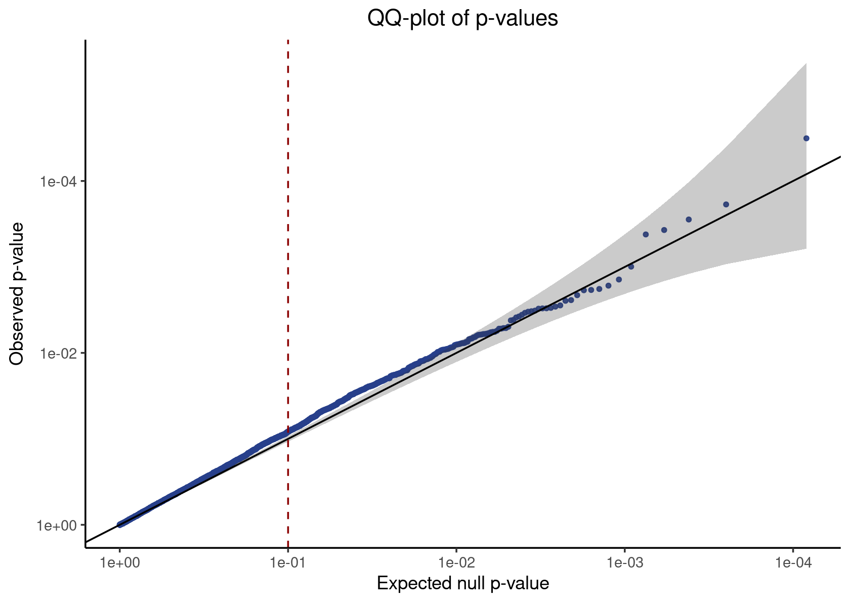
| Version | Author | Date |
|---|---|---|
| e84ebd8 | kevinlkx | 2022-05-26 |
Candidate pairs We extract the p-values corresponding to the candidate pairs and apply a Benjamini-Hochberg (BH) correction to adjust for multiple testing.
simulated_candidate_pair_results <- simulated_result %>% filter(pair_type == "candidate")
simulated_candidate_pair_results_p_adj <- simulated_candidate_pair_results %>%
  mutate(p_val_adj = p.adjust(p_value, method = "BH"))
head(simulated_candidate_pair_results_p_adj)
#           gene_id gRNA_id pair_type    p_value    z_value p_val_adj
# 1 ENSG00000251562  ARID1A candidate 0.04974315 -4.0650638 0.7177451
# 2 ENSG00000271503  ARID1A candidate 0.08164699 -4.7379535 0.7733805
# 3 ENSG00000205542  ARID1A candidate 0.03602927 -2.0986917 0.6886414
# 4 ENSG00000197061  ARID1A candidate 0.63985357  1.3499471 0.9607658
# 5 ENSG00000166710  ARID1A candidate 0.61145577 -0.4742834 0.9584866
# 6 ENSG00000034510  ARID1A candidate 0.69308741 -0.4227958 0.9673933
We call pairs with an adjusted p-value of less or equal than 0.1 significant; the discovery set (i.e., the set of significant pairs) has a false discovery rate (FDR) of 10%.
simulated_discovery_set <- simulated_candidate_pair_results_p_adj %>% filter(p_val_adj <= 0.1)
head(simulated_discovery_set)
#           gene_id gRNA_id pair_type      p_value   z_value    p_val_adj
# 1 ENSG00000019582  ARID1A candidate 7.111315e-05  7.237385 0.0711131498
# 2 ENSG00000277734  ARID1A candidate 2.392761e-05 -5.749545 0.0333873558
# 3 ENSG00000171476  ARID1A candidate 6.543151e-06 -6.836853 0.0137750554
# 4 ENSG00000142546  ARID1A candidate 8.094629e-05  4.973680 0.0758871486
# 5 ENSG00000142669  ARID1A candidate 5.941077e-08 -5.755366 0.0002547392
# 6 ENSG00000172543  ARID1A candidate 3.492456e-05 -6.783390 0.0441152381
saveRDS(simulated_candidate_pair_results_p_adj, file.path(outdir, 'sceptre.candidate.pair.results.rds'))
saveRDS(simulated_discovery_set, file.path(outdir, 'sceptre.discovery.set.results.rds'))Unstimulated T cells
outdir <- '/project2/xinhe/kevinluo/GSFA/sceptre_analysis/TCells_cropseq_data/unsimulated_data/sceptre_output'
unsimulated_result <- readRDS(file.path(outdir, 'sceptre.result.rds'))
head(unsimulated_result, 10)
#            gene_id gRNA_id pair_type     p_value      z_value
# 1  ENSG00000251562  ARID1A candidate 0.307288436 -1.119783084
# 2  ENSG00000271503  ARID1A candidate 0.255094569 -3.434577254
# 3  ENSG00000205542  ARID1A candidate 0.124270007 -1.408917138
# 4  ENSG00000197061  ARID1A candidate 0.508142785  1.959389328
# 5  ENSG00000166710  ARID1A candidate 0.998544879  0.001743273
# 6  ENSG00000034510  ARID1A candidate 0.536159905  0.787584531
# 7  ENSG00000123416  ARID1A candidate 0.828083765 -0.868736493
# 8  ENSG00000100097  ARID1A candidate 0.009152439 -6.235823985
# 9  ENSG00000227507  ARID1A candidate 0.698088383  0.653613012
# 10 ENSG00000115523  ARID1A candidate 0.656404329  2.593409372
Negative control pairs
neg_control_p_vals <- unsimulated_result %>% filter(pair_type == "negative_control") %>% pull(p_value)
qq_plot <- make_qq_plot(neg_control_p_vals)
plot(qq_plot)
| Version | Author | Date |
|---|---|---|
| e84ebd8 | kevinlkx | 2022-05-26 |
Candidate pairs We extract the p-values corresponding to the candidate pairs and apply a Benjamini-Hochberg (BH) correction to adjust for multiple testing.
unsimulated_candidate_pair_results <- unsimulated_result %>% filter(pair_type == "candidate")
unsimulated_candidate_pair_results_p_adj <- unsimulated_candidate_pair_results %>%
  mutate(p_val_adj = p.adjust(p_value, method = "BH"))
head(unsimulated_candidate_pair_results_p_adj)
#           gene_id gRNA_id pair_type   p_value      z_value p_val_adj
# 1 ENSG00000251562  ARID1A candidate 0.3072884 -1.119783084 0.9364386
# 2 ENSG00000271503  ARID1A candidate 0.2550946 -3.434577254 0.9230442
# 3 ENSG00000205542  ARID1A candidate 0.1242700 -1.408917138 0.8776804
# 4 ENSG00000197061  ARID1A candidate 0.5081428  1.959389328 0.9666872
# 5 ENSG00000166710  ARID1A candidate 0.9985449  0.001743273 0.9998483
# 6 ENSG00000034510  ARID1A candidate 0.5361599  0.787584531 0.9711391
We call pairs with an adjusted p-value of less or equal than 0.1 significant; the discovery set (i.e., the set of significant pairs) has a false discovery rate (FDR) of 10%.
unsimulated_discovery_set <- unsimulated_candidate_pair_results_p_adj %>% filter(p_val_adj <= 0.1)
head(unsimulated_discovery_set)
#           gene_id  gRNA_id pair_type      p_value   z_value   p_val_adj
# 1 ENSG00000163191   ARID1A candidate 9.474409e-06 -5.118703 0.031475343
# 2 ENSG00000157303     BTLA candidate 3.239915e-05  4.278822 0.066774171
# 3 ENSG00000146066 C10orf54 candidate 1.075991e-05  4.393335 0.033672848
# 4 ENSG00000043462 C10orf54 candidate 3.060097e-05  4.280412 0.066774171
# 5 ENSG00000117859 C10orf54 candidate 2.915000e-05  4.015791 0.065405999
# 6 ENSG00000167286     CD3D candidate 4.442419e-07 -4.908626 0.002401329
saveRDS(unsimulated_candidate_pair_results_p_adj, file.path(outdir, 'sceptre.candidate.pair.results.rds'))
saveRDS(unsimulated_discovery_set, file.path(outdir, 'sceptre.discovery.set.results.rds'))
sessionInfo()
# R version 4.0.4 (2021-02-15)
# Platform: x86_64-pc-linux-gnu (64-bit)
# Running under: Scientific Linux 7.4 (Nitrogen)
#
# Matrix products: default
# BLAS/LAPACK: /software/openblas-0.3.13-el7-x86_64/lib/libopenblas_haswellp-r0.3.13.so
#
# locale:
#  [1] LC_CTYPE=en_US.UTF-8       LC_NUMERIC=C
#  [3] LC_TIME=en_US.UTF-8        LC_COLLATE=en_US.UTF-8
#  [5] LC_MONETARY=en_US.UTF-8    LC_MESSAGES=en_US.UTF-8
#  [7] LC_PAPER=en_US.UTF-8       LC_NAME=C
#  [9] LC_ADDRESS=C               LC_TELEPHONE=C
# [11] LC_MEASUREMENT=en_US.UTF-8 LC_IDENTIFICATION=C
#
# attached base packages:
# [1] stats     graphics  grDevices utils     datasets  methods   base
#
# other attached packages:
#  [1] SeuratObject_4.0.4 Seurat_4.1.0       sceptre_0.1.0      Matrix_1.4-1
#  [5] cowplot_1.1.1      forcats_0.5.1      stringr_1.4.0      dplyr_1.0.8
#  [9] purrr_0.3.4        readr_2.1.2        tidyr_1.2.0        tibble_3.1.6
# [13] ggplot2_3.3.5      tidyverse_1.3.1    workflowr_1.7.0
#
# loaded via a namespace (and not attached):
#   [1] readxl_1.4.0          backports_1.4.1       plyr_1.8.6
#   [4] igraph_1.2.11         lazyeval_0.2.2        splines_4.0.4
#   [7] listenv_0.8.0         scattermore_0.7       digest_0.6.29
#  [10] htmltools_0.5.2       fansi_1.0.3           magrittr_2.0.3
#  [13] tensor_1.5            cluster_2.1.2         ROCR_1.0-11
#  [16] tzdb_0.3.0            globals_0.14.0        modelr_0.1.8
#  [19] matrixStats_0.61.0    spatstat.sparse_2.1-0 colorspace_2.0-3
#  [22] rvest_1.0.2           ggrepel_0.9.1         haven_2.5.0
#  [25] xfun_0.30             callr_3.7.0           crayon_1.5.1
#  [28] jsonlite_1.8.0        spatstat.data_2.1-2   survival_3.3-1
#  [31] zoo_1.8-9             glue_1.6.2            polyclip_1.10-0
#  [34] gtable_0.3.0          leiden_0.3.9          future.apply_1.8.1
#  [37] abind_1.4-5           scales_1.2.0          DBI_1.1.2
#  [40] spatstat.random_2.1-0 miniUI_0.1.1.1        Rcpp_1.0.8.3
#  [43] viridisLite_0.4.0     xtable_1.8-4          reticulate_1.24
#  [46] spatstat.core_2.4-0   htmlwidgets_1.5.4     httr_1.4.2
#  [49] RColorBrewer_1.1-3    ellipsis_0.3.2        ica_1.0-2
#  [52] farver_2.1.0          pkgconfig_2.0.3       sass_0.4.1
#  [55] uwot_0.1.11           dbplyr_2.1.1          deldir_1.0-6
#  [58] utf8_1.2.2            tidyselect_1.1.2      rlang_1.0.2
#  [61] reshape2_1.4.4        later_1.3.0           munsell_0.5.0
#  [64] cellranger_1.1.0      tools_4.0.4           cli_3.2.0
#  [67] generics_0.1.2        broom_0.8.0           ggridges_0.5.3
#  [70] evaluate_0.15         fastmap_1.1.0         yaml_2.3.5
#  [73] goftest_1.2-3         processx_3.5.3        knitr_1.38
#  [76] fs_1.5.2              fitdistrplus_1.1-8    RANN_2.6.1
#  [79] pbapply_1.5-0         future_1.24.0         nlme_3.1-155
#  [82] whisker_0.4           mime_0.12             xml2_1.3.3
#  [85] compiler_4.0.4        rstudioapi_0.13       plotly_4.10.0
#  [88] png_0.1-7             spatstat.utils_2.3-0  reprex_2.0.1
#  [91] bslib_0.3.1           stringi_1.7.6         highr_0.9
#  [94] ps_1.6.0              lattice_0.20-45       vctrs_0.4.1
#  [97] pillar_1.7.0          lifecycle_1.0.1       spatstat.geom_2.3-2
# [100] lmtest_0.9-40         jquerylib_0.1.4       RcppAnnoy_0.0.19
# [103] data.table_1.14.2     irlba_2.3.5           httpuv_1.6.5
# [106] patchwork_1.1.1       R6_2.5.1              promises_1.2.0.1
# [109] KernSmooth_2.23-20    gridExtra_2.3         parallelly_1.31.0
# [112] codetools_0.2-18      MASS_7.3-56           assertthat_0.2.1
# [115] rprojroot_2.0.2       withr_2.5.0           sctransform_0.3.3
# [118] mgcv_1.8-39           parallel_4.0.4        hms_1.1.1
# [121] grid_4.0.4            rpart_4.1-15          rmarkdown_2.13
# [124] Rtsne_0.15            git2r_0.30.1          getPass_0.2-2
# [127] shiny_1.7.1           lubridate_1.8.0