MUSIC analysis on CD8+ T Cell (stimulated and unstimulated) CROP-seq data
Kaixuan Luo
2022-07-14
Last updated: 2022-09-20
Checks: 7 0
Knit directory: GSFA_analysis/
This reproducible R Markdown analysis was created with workflowr (version 1.7.0). The Checks tab describes the reproducibility checks that were applied when the results were created. The Past versions tab lists the development history.
Great! Since the R Markdown file has been committed to the Git repository, you know the exact version of the code that produced these results.
Great job! The global environment was empty. Objects defined in the global environment can affect the analysis in your R Markdown file in unknown ways. For reproduciblity it’s best to always run the code in an empty environment.
The command set.seed(20220524) was run prior to running
the code in the R Markdown file. Setting a seed ensures that any results
that rely on randomness, e.g. subsampling or permutations, are
reproducible.
Great job! Recording the operating system, R version, and package versions is critical for reproducibility.
Nice! There were no cached chunks for this analysis, so you can be confident that you successfully produced the results during this run.
Great job! Using relative paths to the files within your workflowr project makes it easier to run your code on other machines.
Great! You are using Git for version control. Tracking code development and connecting the code version to the results is critical for reproducibility.
The results in this page were generated with repository version 4a35fbe. See the Past versions tab to see a history of the changes made to the R Markdown and HTML files.
Note that you need to be careful to ensure that all relevant files for
the analysis have been committed to Git prior to generating the results
(you can use wflow_publish or
wflow_git_commit). workflowr only checks the R Markdown
file, but you know if there are other scripts or data files that it
depends on. Below is the status of the Git repository when the results
were generated:
Ignored files:
    Ignored:    .DS_Store
    Ignored:    .Rhistory
    Ignored:    .Rproj.user/

Untracked files:
    Untracked:  Rplots.pdf
    Untracked:  analysis/check_Tcells_datasets.Rmd
    Untracked:  analysis/fscLVM_analysis.Rmd
    Untracked:  analysis/spca_LUHMES_data.Rmd
    Untracked:  analysis/test_seurat.Rmd
    Untracked:  code/gsfa_negctrl_job.sbatch
    Untracked:  code/music_LUHMES_Yifan.R
    Untracked:  code/plotting_functions.R
    Untracked:  code/run_fscLVM_LUHMES_data.R
    Untracked:  code/run_gsfa_2groups_negctrl.R
    Untracked:  code/run_gsfa_negctrl.R
    Untracked:  code/run_music_LUHMES.R
    Untracked:  code/run_music_LUHMES_data.sbatch
    Untracked:  code/run_music_LUHMES_data_20topics.R
    Untracked:  code/run_music_LUHMES_data_20topics.sbatch
    Untracked:  code/run_sceptre_Tcells_data.sbatch
    Untracked:  code/run_sceptre_Tcells_stimulated_data.sbatch
    Untracked:  code/run_sceptre_Tcells_test_data.sbatch
    Untracked:  code/run_sceptre_Tcells_unstimulated_data.sbatch
    Untracked:  code/run_sceptre_permuted_data.sbatch
    Untracked:  code/run_spca_LUHMES.R
    Untracked:  code/run_spca_TCells.R
    Untracked:  code/run_twostep_clustering_LUHMES_data.sbatch
    Untracked:  code/run_twostep_clustering_Tcells_data.sbatch
    Untracked:  code/run_unguided_gsfa_LUHMES.R
    Untracked:  code/run_unguided_gsfa_LUHMES.sbatch
    Untracked:  code/run_unguided_gsfa_Tcells.R
    Untracked:  code/run_unguided_gsfa_Tcells.sbatch
    Untracked:  code/sceptre_LUHMES_data.R
    Untracked:  code/sceptre_Tcells_stimulated_data.R
    Untracked:  code/sceptre_Tcells_unstimulated_data.R
    Untracked:  code/sceptre_permutation_analysis.R
    Untracked:  code/sceptre_permute_analysis.R
    Untracked:  code/seurat_sim_fpr_tpr.R
    Untracked:  code/unguided_GFSA_mixture_normal_prior.cpp

Unstaged changes:
    Modified:   analysis/music_LUHMES_data.Rmd
    Modified:   analysis/sceptre_TCells_data.Rmd
    Modified:   analysis/twostep_clustering_LUHMES_data.Rmd
    Modified:   code/run_sceptre_LUHMES_data.R
    Modified:   code/run_sceptre_LUHMES_data.sbatch
    Modified:   code/run_sceptre_LUHMES_permuted_data.R
    Modified:   code/run_sceptre_Tcells_permuted_data.R
    Modified:   code/run_sceptre_cropseq_data.sbatch
    Modified:   code/run_twostep_clustering_LUHMES_data.R
    Modified:   code/sceptre_analysis.R
Note that any generated files, e.g. HTML, png, CSS, etc., are not included in this status report because it is ok for generated content to have uncommitted changes.
These are the previous versions of the repository in which changes were
made to the R Markdown (analysis/music_TCells_data.Rmd) and
HTML (docs/music_TCells_data.html) files. If you’ve
configured a remote Git repository (see ?wflow_git_remote),
click on the hyperlinks in the table below to view the files as they
were in that past version.
| File | Version | Author | Date | Message |
|---|---|---|---|---|
| Rmd | 4a35fbe | kevinlkx | 2022-09-20 | updated dot plots |
| html | b9fac2b | kevinlkx | 2022-09-20 | Build site. |
| Rmd | 6e34d2c | kevinlkx | 2022-09-20 | updated dot plots |
| html | 054f057 | kevinlkx | 2022-08-11 | Build site. |
| Rmd | b7ce856 | kevinlkx | 2022-08-11 | fix intro formatting |
| html | b1684a9 | kevinlkx | 2022-08-11 | Build site. |
| Rmd | 1429b75 | kevinlkx | 2022-08-11 | added dot plots with Bonferroni adjusted p-value |
| html | 069e245 | kevinlkx | 2022-07-29 | Build site. |
| Rmd | ee2a305 | kevinlkx | 2022-07-29 | update doplot figure legend |
| html | 2625955 | kevinlkx | 2022-07-29 | Build site. |
| Rmd | 87e2aa2 | kevinlkx | 2022-07-29 | updated links to R scripts |
| html | 7102e1b | kevinlkx | 2022-07-29 | Build site. |
| Rmd | 2bf6abd | kevinlkx | 2022-07-29 | added dotplots with MUSIC empirical TPD FDR |
| html | d3e54fd | kevinlkx | 2022-07-25 | Build site. |
| Rmd | 3178265 | kevinlkx | 2022-07-25 | update music results for T cells |
MUSIC website: https://github.com/bm2-lab/MUSIC
Scripts for running the analysis:
Stimulated data:
Unstimulated data:
cd /project2/xinhe/kevinluo/GSFA/music_analysis/log

sbatch --mem=50G --cpus-per-task=5 ~/projects/GSFA_analysis/code/run_music_Tcells_stimulated_data.sbatch

sbatch --mem=50G --cpus-per-task=5 ~/projects/GSFA_analysis/code/run_music_Tcells_unstimulated_data.sbatch
Load packages
dyn.load('/software/geos-3.7.0-el7-x86_64/lib64/libgeos_c.so') # attach the geos lib for Seurat
suppressPackageStartupMessages(library(data.table))
suppressPackageStartupMessages(library(Seurat))
suppressPackageStartupMessages(library(MUSIC))
suppressPackageStartupMessages(library(ComplexHeatmap))
suppressPackageStartupMessages(library(ggplot2))
theme_set(theme_bw() + theme(plot.title = element_text(size = 14, hjust = 0.5),
                             axis.title = element_text(size = 14),
                             axis.text = element_text(size = 13),
                             legend.title = element_text(size = 13),
                             legend.text = element_text(size = 12),
                             panel.grid.minor = element_blank())
)

source("code/plotting_functions.R")
Functions
## Adapted over MUSIC's Diff_topic_distri() function
Empirical_topic_prob_diff <- function(model, perturb_information,
                                      permNum = 10^4, seed = 1000){
  require(reshape2)
  require(dplyr)
  require(ComplexHeatmap)
  options(warn = -1)
  prob_mat <- model@gamma
  row.names(prob_mat) <- model@documents
  topicNum <- ncol(prob_mat)
  topicName <- paste0('Topic_', 1:topicNum)
  colnames(prob_mat) <- topicName
  ko_name <- unique(perturb_information)
  prob_df <- data.frame(prob_mat,
                        samples = rownames(prob_mat),
                        knockout = perturb_information)

  prob_df <- melt(prob_df, id = c('samples', 'knockout'), variable.name = "topic")

  summary_df <- prob_df %>%
    group_by(knockout, topic) %>%
    summarise(number = sum(value)) %>%
    ungroup() %>%
    group_by(knockout) %>%
    mutate(cellNum = sum(number)) %>%
    ungroup() %>%
    mutate(ratio = number/cellNum)

  summary_df$ctrlNum <- rep(summary_df$cellNum[summary_df$knockout == "CTRL"],
                            length(ko_name))
  summary_df$ctrl_ratio <- rep(summary_df$ratio[summary_df$knockout == "CTRL"],
                               length(ko_name))
  summary_df <- summary_df %>% mutate(diff_index = ratio - ctrl_ratio)

  test_df <- data.frame(matrix(nrow = length(ko_name) * topicNum, ncol = 5))
  colnames(test_df) <- c("knockout", "topic", "obs_t_stats", "obs_pval", "empirical_pval")
  k <- 1
  for(i in topicName){
    prob_df.topic <- prob_df[prob_df$topic == i, ]
    ctrl_topic <- prob_df.topic$value[prob_df.topic$knockout == "CTRL"]
    ctrl_topic_z <- (ctrl_topic - mean(ctrl_topic)) / sqrt(var(ctrl_topic))
    for(j in ko_name){
      ko_topic <- prob_df.topic$value[prob_df.topic$knockout == j]
      ko_topic_z <- (ko_topic - mean(ctrl_topic)) / sqrt(var(ctrl_topic))
      test_df$knockout[k] <- j
      test_df$topic[k] <- i
      test <- t.test(ko_topic_z, ctrl_topic_z)
      test_df$obs_t_stats[k] <- test$statistic
      test_df$obs_pval[k] <- test$p.value
      k <- k + 1
    }
  }

  ## Permutation on the perturbation conditions:
  # permNum <- 10^4
  print(paste0("Performing permutation for ", permNum, " rounds."))
  perm_t_stats <- matrix(0, nrow = nrow(test_df), ncol = permNum)
  set.seed(seed)
  for (perm in 1:permNum){
    perm_prob_df <- data.frame(prob_mat,
                               samples = rownames(prob_mat),
                               knockout = perturb_information[sample(length(perturb_information))])
    perm_prob_df <- melt(perm_prob_df, id = c('samples', 'knockout'), variable.name = "topic")
    k <- 1
    for(i in topicName){
      perm_prob_df.topic <- perm_prob_df[perm_prob_df$topic == i, ]
      ctrl_topic <- perm_prob_df.topic$value[perm_prob_df.topic$knockout == "CTRL"]
      ctrl_topic_z <- (ctrl_topic - mean(ctrl_topic)) / sqrt(var(ctrl_topic))
      for(j in ko_name){
        ko_topic <- perm_prob_df.topic$value[perm_prob_df.topic$knockout == j]
        ko_topic_z <- (ko_topic - mean(ctrl_topic)) / sqrt(var(ctrl_topic))
        test <- t.test(ko_topic_z, ctrl_topic_z)
        perm_t_stats[k, perm] <- test$statistic
        k <- k + 1
      }
    }
    if (perm %% 1000 == 0){
      print(paste0(perm, " rounds finished."))
    }
  }
  ## Compute two-sided empirical p value:
  for (k in 1:nrow(test_df)){
    test_df$empirical_pval[k] <-
      2 * min(mean(perm_t_stats[k, ] <= test_df$obs_t_stats[k]),
              mean(perm_t_stats[k, ] >= test_df$obs_t_stats[k]))
  }
  test_df <- test_df %>%
    mutate(empirical_pval = ifelse(empirical_pval == 0, 1/permNum, empirical_pval)) %>%
    mutate(empirical_pval = ifelse(empirical_pval > 1, 1, empirical_pval))

  summary_df <- inner_join(summary_df, test_df, by = c("knockout", "topic"))
  summary_df <- summary_df %>%
    mutate(polar_log10_pval = ifelse(obs_t_stats > 0, -log10(empirical_pval), log10(empirical_pval)))
  return(summary_df)
}
About the data sets
CROP-seq datasets:
/project2/xinhe/yifan/Factor_analysis/shared_data/. The
data are Seurat objects, with raw gene counts stored in
obj@assays$RNA@counts, and cell meta data stored in
obj@meta.data. Normalized and scaled data used for GSFA are
stored in obj@assays$RNA@scale.data, the rownames of which
are the 6k genes used for GSFA.
Set directories
data_dir <- "/project2/xinhe/yifan/Factor_analysis/Stimulated_T_Cells/"
dir.create("/project2/xinhe/kevinluo/GSFA/music_analysis/Stimulated_T_Cells", recursive = TRUE, showWarnings = FALSE)
Load the T Cells CROP-seq data
combined_obj <- readRDS('/project2/xinhe/yifan/Factor_analysis/shared_data/TCells_cropseq_data_seurat.rds')Separate stimulated and unstimulated cells into two data sets, and run those separately.
metadata <- combined_obj@meta.data
metadata[1:5, ]

table(metadata$orig.ident)

stimulated_cells <- rownames(metadata)[which(endsWith(metadata$orig.ident, "S"))]
cat(length(stimulated_cells), "stimulated cells. \n")
unstimulated_cells <- rownames(metadata)[which(endsWith(metadata$orig.ident, "N"))]
cat(length(unstimulated_cells), "unstimulated cells. \n")
orig.ident nCount_RNA nFeature_RNA ARID1A BTLA C10orf54
D1S_AAACCTGAGCGATTCT TCells_D1S 8722 2642 0 0 0
D1S_AAACCTGCAAGCCGTC TCells_D1S 7296 2356 0 1 0
D1S_AAACCTGCAGGGCATA TCells_D1S 6467 2154 0 0 0
D1S_AAACCTGGTAAGGGCT TCells_D1S 12151 3121 0 0 0
D1S_AAACCTGGTAGCGCTC TCells_D1S 11170 2964 0 0 1
CBLB CD3D CD5 CDKN1B DGKA DGKZ HAVCR2 LAG3 LCP2 MEF2D
D1S_AAACCTGAGCGATTCT 0 0 0 0 0 0 0 0 0 0
D1S_AAACCTGCAAGCCGTC 0 0 0 0 0 0 0 0 0 0
D1S_AAACCTGCAGGGCATA 0 0 0 0 0 0 0 0 0 0
D1S_AAACCTGGTAAGGGCT 1 0 0 0 0 0 0 0 0 0
D1S_AAACCTGGTAGCGCTC 0 0 0 0 0 0 0 0 0 0
NonTarget PDCD1 RASA2 SOCS1 STAT6 TCEB2 TMEM222 TNFRSF9
D1S_AAACCTGAGCGATTCT 0 0 0 0 0 1 0 0
D1S_AAACCTGCAAGCCGTC 0 0 0 0 0 0 0 0
D1S_AAACCTGCAGGGCATA 0 0 0 0 1 0 0 0
D1S_AAACCTGGTAAGGGCT 0 0 0 0 0 0 0 0
D1S_AAACCTGGTAGCGCTC 0 0 0 0 0 0 0 0
percent_mt gRNA_umi_count
D1S_AAACCTGAGCGATTCT 3.370787 1
D1S_AAACCTGCAAGCCGTC 5.921053 1
D1S_AAACCTGCAGGGCATA 2.860677 1
D1S_AAACCTGGTAAGGGCT 3.045017 6
D1S_AAACCTGGTAGCGCTC 3.240824 7
TCells_D1N TCells_D1S TCells_D2N TCells_D2S
5533 6843 5144 7435
14278 stimulated cells.
10677 unstimulated cells. Run simulated data
dir.create("/project2/xinhe/kevinluo/GSFA/music_analysis/Stimulated_T_Cells/stimulated", recursive = TRUE, showWarnings = FALSE)
res_dir <- "/project2/xinhe/kevinluo/GSFA/music_analysis/Stimulated_T_Cells/stimulated"
dir.create(file.path(res_dir,"/music_output"), recursive = TRUE, showWarnings = FALSE)setwd(res_dir)0. Load input data
feature.names <- data.frame(fread(paste0(data_dir, "GSE119450_RAW/D1N/genes.tsv"),
                                  header = FALSE), stringsAsFactors = FALSE)

expression_profile <- combined_obj@assays$RNA@counts[, stimulated_cells]
rownames(expression_profile) <- feature.names$V2[match(rownames(expression_profile),
                                                       feature.names$V1)]
cat("Dimension of expression profile matrix: \n")
dim(expression_profile)

targets <- names(combined_obj@meta.data)[4:24]
targets[targets == "NonTarget"] <- "CTRL"
cat("Targets: \n")
print(targets)

perturb_information <- apply(combined_obj@meta.data[stimulated_cells, 4:24], 1,
                             function(x){ targets[which(x > 0)] })
Dimension of expression profile matrix:
[1] 33694 14278
Targets:
[1] "ARID1A" "BTLA" "C10orf54" "CBLB" "CD3D" "CD5"
[7] "CDKN1B" "DGKA" "DGKZ" "HAVCR2" "LAG3" "LCP2"
[13] "MEF2D" "CTRL" "PDCD1" "RASA2" "SOCS1" "STAT6"
[19] "TCEB2" "TMEM222" "TNFRSF9" 1. Data preprocessing
crop_seq_list <- Input_preprocess(expression_profile, perturb_information)

crop_seq_qc <- Cell_qc(crop_seq_list$expression_profile,
                       crop_seq_list$perturb_information,
                       species = "Hs", plot = F)
saveRDS(crop_seq_qc, "music_output/music_crop_seq_qc.rds")

crop_seq_imputation <- Data_imputation(crop_seq_qc$expression_profile,
                                       crop_seq_qc$perturb_information,
                                       cpu_num = 5)
saveRDS(crop_seq_imputation, "music_output/music_imputation.merged.rds")

crop_seq_filtered <- Cell_filtering(crop_seq_imputation$expression_profile,
                                    crop_seq_imputation$perturb_information,
                                    cpu_num = 5)
saveRDS(crop_seq_filtered, "music_output/music_filtered.merged.rds")
2. Model building
crop_seq_vargene <- Get_high_varGenes(crop_seq_filtered$expression_profile,
                                      crop_seq_filtered$perturb_information, plot = T)
saveRDS(crop_seq_vargene, "music_output/music_vargene.merged.rds")

crop_seq_vargene <- readRDS("music_output/music_vargene.merged.rds")

## Get_topics() can take up to a few hours to finish,
## depending on the size of data
system.time(
  topic_1 <- Get_topics(crop_seq_vargene$expression_profile,
                        crop_seq_vargene$perturb_information,
                        topic_number = 5))
saveRDS(topic_1, "music_output/music_merged_5_topics.rds")

system.time(
  topic_2 <- Get_topics(crop_seq_vargene$expression_profile,
                        crop_seq_vargene$perturb_information,
                        topic_number = 10))
saveRDS(topic_2, "music_output/music_merged_10_topics.rds")

system.time(
  topic_3 <- Get_topics(crop_seq_vargene$expression_profile,
                        crop_seq_vargene$perturb_information,
                        topic_number = 15))
saveRDS(topic_3, "music_output/music_merged_15_topics.rds")

system.time(
  topic_4 <- Get_topics(crop_seq_vargene$expression_profile,
                        crop_seq_vargene$perturb_information,
                        topic_number = 20))
saveRDS(topic_4, "music_output/music_merged_20_topics.rds")

## try fewer numbers of topics
system.time(
  topic_5 <- Get_topics(crop_seq_vargene$expression_profile,
                        crop_seq_vargene$perturb_information,
                        topic_number = 4))
saveRDS(topic_5, "music_output/music_merged_4_topics.rds")

system.time(
  topic_6 <- Get_topics(crop_seq_vargene$expression_profile,
                        crop_seq_vargene$perturb_information,
                        topic_number = 6))
saveRDS(topic_6, "music_output/music_merged_6_topics.rds")
3. Pick the number of topics
topic_1 <- readRDS("music_output/music_merged_4_topics.rds")
topic_2 <- readRDS("music_output/music_merged_5_topics.rds")
topic_3 <- readRDS("music_output/music_merged_6_topics.rds")
topic_4 <- readRDS("music_output/music_merged_10_topics.rds")
topic_5 <- readRDS("music_output/music_merged_15_topics.rds")
topic_6 <- readRDS("music_output/music_merged_20_topics.rds")

topic_model_list <- list()
topic_model_list$models <- list()
topic_model_list$perturb_information <- topic_1$perturb_information
topic_model_list$models[[1]] <- topic_1$models[[1]]
topic_model_list$models[[2]] <- topic_2$models[[1]]
topic_model_list$models[[3]] <- topic_3$models[[1]]
topic_model_list$models[[4]] <- topic_4$models[[1]]
topic_model_list$models[[5]] <- topic_5$models[[1]]
topic_model_list$models[[6]] <- topic_6$models[[1]]

optimalModel <- Select_topic_number(topic_model_list$models,
                                    plot = T,
                                    plot_path = "music_output/select_topic_number_4to6to20.pdf")
Summarize the results
Summarize the results under 20 topics to be comparable to GSFA
Gene ontology annotations for top topics
topic_res <- readRDS("music_output/music_merged_20_topics.rds")

topic_func <- Topic_func_anno(topic_res$models[[1]], species = "Hs")
saveRDS(topic_func, "music_output/topic_func_20_topics.rds")
topic_func <- readRDS("music_output/topic_func_20_topics.rds")
pdf("music_output/music_merged_20_topics_GO_annotations.pdf",
width = 14, height = 12)
ggplot(topic_func$topic_annotation_result) +
geom_point(aes(x = Cluster, y = Description,
size = Count, color = -log10(qvalue))) +
scale_color_gradientn(colors = c("blue", "red")) +
theme_bw() +
theme(axis.title = element_blank(),
axis.text.x = element_text(angle = 45, hjust = 1))
dev.off()Perturbation effect prioritizing
# calculate topic distribution for each cell.
distri_diff <- Diff_topic_distri(topic_res$models[[1]],
                                 topic_res$perturb_information,
                                 plot = T)
# saveRDS(distri_diff, "music_output/distri_diff_20_topics.rds")

distri_diff <- readRDS("music_output/distri_diff_20_topics.rds")
t_D_diff_matrix <- dcast(distri_diff %>% dplyr::select(knockout, variable, t_D_diff),
                         knockout ~ variable)
rownames(t_D_diff_matrix) <- t_D_diff_matrix$knockout
t_D_diff_matrix$knockout <- NULL
pdf("music_output/music_merged_20_topics_TPD_heatmap.pdf", width = 12, height = 8)
Heatmap(t_D_diff_matrix,
name = "Topic probability difference (vs ctrl)",
cluster_rows = T, cluster_columns = T,
column_names_rot = 45,
heatmap_legend_param = list(title_gp = gpar(fontsize = 12, fontface = "bold")))
dev.off()Calculate the overall perturbation effect ranking list without “offTarget_Info”.
distri_diff <- readRDS(file.path(res_dir, "music_output/distri_diff_20_topics.rds"))

rank_overall_result <- Rank_overall(distri_diff)
print(rank_overall_result)
# saveRDS(rank_overall_result, "music_output/rank_overall_result_20_topics.rds")
perturbation ranking Score off_target
1 CD3D 1 207.89434 none
2 CBLB 2 181.54109 none
3 HAVCR2 3 164.90364 none
4 MEF2D 4 159.47255 none
5 LAG3 5 146.92054 none
6 LCP2 6 142.39084 none
7 TMEM222 7 131.76594 none
8 RASA2 8 123.32882 none
9 PDCD1 9 117.64996 none
10 TNFRSF9 10 102.44654 none
11 CD5 11 100.44077 none
12 SOCS1 12 97.63884 none
13 BTLA 13 93.85907 none
14 DGKZ 14 84.20973 none
15 TCEB2 15 75.95113 none
16 ARID1A 16 74.05189 none
17 CDKN1B 17 68.22507 none
18 STAT6 18 41.90055 none
19 DGKA 19 39.74996 none
20 C10orf54 20 31.02633 nonecalculate the topic-specific ranking list.
rank_topic_specific_result <- Rank_specific(distri_diff)
head(rank_topic_specific_result, 10)
# saveRDS(rank_topic_specific_result, "music_output/rank_topic_specific_result_20_topics.rds")
topic perturbation ranking
1 Topic1 LCP2 1
2 Topic1 CD3D 2
3 Topic1 CD5 3
4 Topic1 ARID1A 4
5 Topic1 DGKA 5
6 Topic1 CDKN1B 6
7 Topic1 STAT6 7
8 Topic1 MEF2D 8
9 Topic1 C10orf54 9
10 Topic1 DGKZ 10calculate the perturbation correlation.
perturb_cor <- Correlation_perturbation(distri_diff,
                                        cutoff = 0.5, gene = "all", plot = T,
                                        plot_path = file.path(res_dir, "music_output/correlation_network_20_topics.pdf"))

head(perturb_cor, 10)
# saveRDS(perturb_cor, "music_output/perturb_cor_20_topics.rds")
Perturbation_1 Perturbation_2 Correlation
2 BTLA ARID1A 0.81287901
3 C10orf54 ARID1A 0.35807563
23 C10orf54 BTLA 0.16626640
24 CBLB BTLA -0.53610756
4 CBLB ARID1A -0.08829456
44 CBLB C10orf54 0.04880987
65 CD3D CBLB -0.83212031
25 CD3D BTLA 0.63583820
5 CD3D ARID1A 0.18307594
45 CD3D C10orf54 0.06519028Adaptation to the code to generate calibrated empirical TPD scores
summary_df <- Empirical_topic_prob_diff(topic_res$models[[1]],
                                        topic_res$perturb_information)
saveRDS(summary_df, "music_output/music_merged_20_topics_ttest_summary.rds")
summary_df <- readRDS(file.path(res_dir, "music_output/music_merged_20_topics_ttest_summary.rds"))
summary_df$topic <- gsub("_", " ", summary_df$topic)
summary_df$topic <- factor(summary_df$topic, levels = paste("Topic", 1:length(unique(summary_df$topic))))
summary_df$fdr <- p.adjust(summary_df$empirical_pval, method = "BH")
summary_df$bonferroni_adj <- p.adjust(summary_df$empirical_pval, method = "bonferroni")
log10_pval_mat <- dcast(summary_df %>% dplyr::select(knockout, topic, polar_log10_pval),
knockout ~ topic)
rownames(log10_pval_mat) <- log10_pval_mat$knockout
log10_pval_mat$knockout <- NULL
effect_mat <- dcast(summary_df %>% dplyr::select(knockout, topic, obs_t_stats), knockout ~ topic)
rownames(effect_mat) <- effect_mat$knockout
effect_mat$knockout <- NULL
fdr_mat <- dcast(summary_df %>% dplyr::select(knockout, topic, fdr), knockout ~ topic)
rownames(fdr_mat) <- fdr_mat$knockout
fdr_mat$knockout <- NULL
bonferroni_mat <- dcast(summary_df %>% dplyr::select(knockout, topic, bonferroni_adj), knockout ~ topic)
rownames(bonferroni_mat) <- bonferroni_mat$knockout
bonferroni_mat$knockout <- NULL# pdf("music_output/music_merged_20_topics_empirical_tstats_heatmap.pdf",
# width = 12, height = 8)
ht <- Heatmap(log10_pval_mat,
name = "Polarized empirical t-test -log10(p-value)\n(KO vs ctrl cell topic probs)",
col = circlize::colorRamp2(breaks = c(-4, 0, 4), colors = c("blue", "grey90", "red")),
cluster_rows = T, cluster_columns = T,
column_names_rot = 45,
heatmap_legend_param = list(title_gp = gpar(fontsize = 12,
fontface = "bold")))
draw(ht)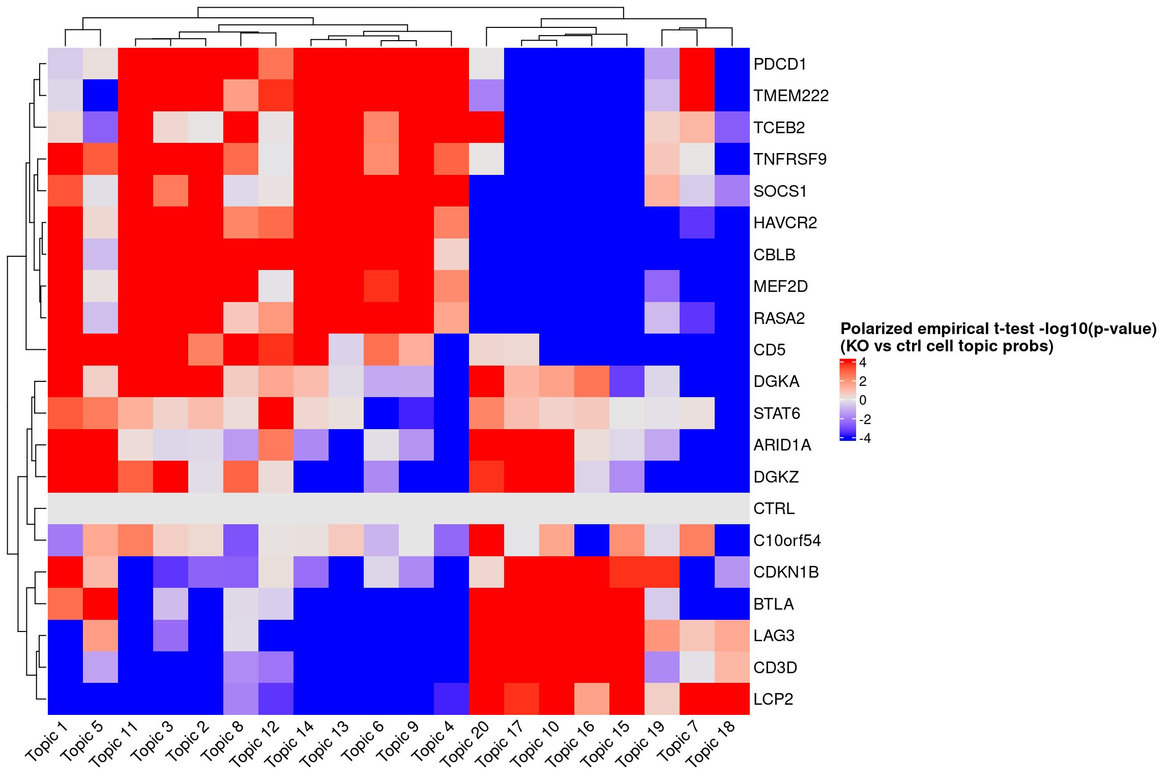
# dev.off()# pdf("music_output/music_merged_20_topics_empirical_tstats_fdr_dotplot.pdf",
# width = 12, height = 8)
KO_names <- rownames(fdr_mat)
dotplot_effectsize(t(effect_mat), t(fdr_mat),
reorder_markers = c(KO_names[KO_names!="CTRL"], "CTRL"),
color_lgd_title = "MUSIC T statistics",
size_lgd_title = "FDR",
max_score = 20,
min_score = -20,
by_score = 10) +
coord_flip() +
theme(axis.text.x = element_text(angle = 45, vjust = 1))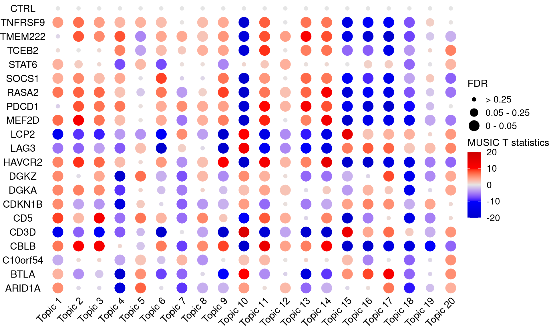
# dev.off()KO_names <- rownames(bonferroni_mat)
dotplot_effectsize(t(effect_mat), t(bonferroni_mat),
reorder_markers = c(KO_names[KO_names!="CTRL"], "CTRL"),
color_lgd_title = "MUSIC T statistics",
size_lgd_title = "Bonferroni\nadjusted p-value",
max_score = 20,
min_score = -20,
by_score = 10) +
coord_flip() +
theme(axis.text.x = element_text(angle = 45, vjust = 1, hjust = 1))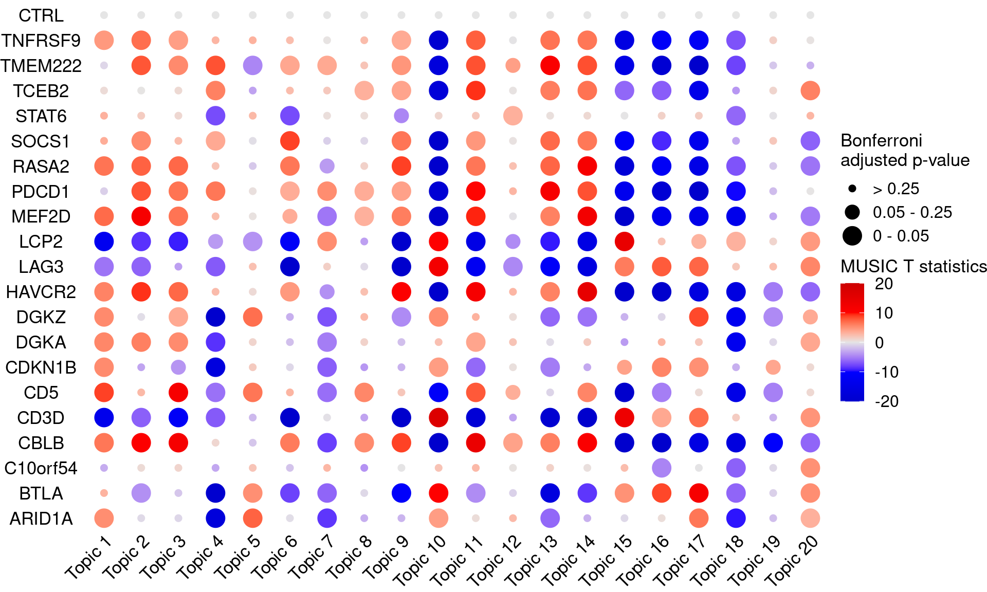
Summarize the results using the optimal number of topics selected by the score
topic_1 <- readRDS("music_output/music_merged_4_topics.rds")
topic_2 <- readRDS("music_output/music_merged_5_topics.rds")
topic_3 <- readRDS("music_output/music_merged_6_topics.rds")

topic_model_list <- list()
topic_model_list$models <- list()
topic_model_list$perturb_information <- topic_1$perturb_information
topic_model_list$models[[1]] <- topic_1$models[[1]]
topic_model_list$models[[2]] <- topic_2$models[[1]]
topic_model_list$models[[3]] <- topic_3$models[[1]]

optimalModel <- Select_topic_number(topic_model_list$models,
                                    plot = T,
                                    plot_path = "music_output/select_topic_number_4to6.pdf")
optimalModel
saveRDS(optimalModel, "music_output/optimalModel_4_topics.rds")
Gene ontology annotations for top topics
topic_func <- Topic_func_anno(optimalModel, species = "Hs", plot_path = "music_output/topic_annotation_GO_4_topics.pdf")
saveRDS(topic_func, "music_output/topic_func_4_topics.rds")
topic_func <- readRDS("music_output/topic_func_4_topics.rds")
pdf("music_output/music_merged_4_topics_GO_annotations.pdf",
width = 14, height = 12)
ggplot(topic_func$topic_annotation_result) +
geom_point(aes(x = Cluster, y = Description,
size = Count, color = -log10(qvalue))) +
scale_color_gradientn(colors = c("blue", "red")) +
theme_bw() +
theme(axis.title = element_blank(),
axis.text.x = element_text(angle = 45, hjust = 1))
dev.off()Perturbation effect prioritizing
# calculate topic distribution for each cell.
distri_diff <- Diff_topic_distri(optimalModel,
                                 topic_model_list$perturb_information,
                                 plot = T,
                                 plot_path = "music_output/distribution_of_topic_4_topics.pdf")
saveRDS(distri_diff, "music_output/distri_diff_4_topics.rds")

t_D_diff_matrix <- dcast(distri_diff %>% dplyr::select(knockout, variable, t_D_diff),
                         knockout ~ variable)
rownames(t_D_diff_matrix) <- t_D_diff_matrix$knockout
t_D_diff_matrix$knockout <- NULL
pdf("music_output/music_merged_4_topics_TPD_heatmap.pdf", width = 12, height = 8)
Heatmap(t_D_diff_matrix,
name = "Topic probability difference (vs ctrl)",
cluster_rows = T, cluster_columns = T,
column_names_rot = 45,
heatmap_legend_param = list(title_gp = gpar(fontsize = 12, fontface = "bold")))
dev.off()The overall perturbation effect ranking list.
distri_diff <- readRDS(file.path(res_dir, "music_output/distri_diff_4_topics.rds"))

rank_overall_result <- Rank_overall(distri_diff)
print(rank_overall_result)
# saveRDS(rank_overall_result, "music_output/rank_overall_4_topics_result.rds")
perturbation ranking Score off_target
1 CD3D 1 80.479730 none
2 CBLB 2 60.497307 none
3 HAVCR2 3 56.031576 none
4 MEF2D 4 54.385870 none
5 LAG3 5 53.626918 none
6 LCP2 6 50.550911 none
7 RASA2 7 40.714017 none
8 TMEM222 8 40.266773 none
9 PDCD1 9 33.086684 none
10 SOCS1 10 31.989369 none
11 BTLA 11 31.950377 none
12 TNFRSF9 12 30.519064 none
13 DGKZ 13 28.659389 none
14 CD5 14 28.418794 none
15 TCEB2 15 23.491816 none
16 ARID1A 16 22.865849 none
17 CDKN1B 17 17.677077 none
18 STAT6 18 15.492215 none
19 DGKA 19 13.237648 none
20 C10orf54 20 3.782439 noneTopic-specific ranking list.
rank_topic_specific_result <- Rank_specific(distri_diff)
print(rank_topic_specific_result)
# saveRDS(rank_topic_specific_result, "music_output/rank_topic_specific_4_topics_result.rds")
topic perturbation ranking
1 Topic1 CD3D 1
2 Topic1 MEF2D 2
3 Topic1 CBLB 3
4 Topic1 LCP2 4
5 Topic1 HAVCR2 5
6 Topic2 LAG3 1
7 Topic2 CD3D 2
8 Topic2 LCP2 3
9 Topic2 STAT6 4
10 Topic2 SOCS1 5
11 Topic2 BTLA 6
12 Topic2 RASA2 7
13 Topic2 HAVCR2 8
14 Topic2 CBLB 9
15 Topic2 MEF2D 10
16 Topic2 TMEM222 11
17 Topic2 TCEB2 12
18 Topic2 PDCD1 13
19 Topic2 DGKZ 14
20 Topic2 C10orf54 15
21 Topic2 TNFRSF9 16
22 Topic3 DGKZ 1
23 Topic3 ARID1A 2
24 Topic3 CD5 3
25 Topic3 DGKA 4
26 Topic3 CBLB 5
27 Topic3 BTLA 6
28 Topic3 CDKN1B 7
29 Topic3 C10orf54 8
30 Topic3 STAT6 9
31 Topic3 MEF2D 10
32 Topic3 HAVCR2 11
33 Topic3 LCP2 12
34 Topic3 RASA2 13
35 Topic3 TNFRSF9 14
36 Topic3 TCEB2 15
37 Topic3 TMEM222 16
38 Topic3 CD3D 17
39 Topic3 SOCS1 18
40 Topic3 PDCD1 19
41 Topic3 LAG3 20
42 Topic4 TMEM222 1
43 Topic4 HAVCR2 2
44 Topic4 PDCD1 3
45 Topic4 SOCS1 4
46 Topic4 CBLB 5
47 Topic4 RASA2 6
48 Topic4 MEF2D 7
49 Topic4 TCEB2 8
50 Topic4 BTLA 9
51 Topic4 TNFRSF9 10
52 Topic4 CD3D 11
53 Topic4 CDKN1B 12
54 Topic4 LAG3 13
55 Topic4 ARID1A 14
56 Topic4 DGKZ 15
57 Topic4 LCP2 16
58 Topic4 STAT6 17
59 Topic4 C10orf54 18
60 Topic4 DGKA 19
61 Topic4 CD5 20Perturbation correlation.
perturb_cor <- Correlation_perturbation(distri_diff,
                                        cutoff = 0.5, gene = "all", plot = T,
                                        plot_path = file.path(res_dir, "music_output/correlation_network_4_topics.pdf"))

head(perturb_cor, 10)
# saveRDS(perturb_cor, "music_output/perturb_cor_4_topics.rds")
Perturbation_1 Perturbation_2 Correlation
2 BTLA ARID1A 0.768508989
3 C10orf54 ARID1A 0.876073418
23 C10orf54 BTLA 0.629414928
24 CBLB BTLA -0.613803324
44 CBLB C10orf54 0.225585570
4 CBLB ARID1A -0.052114102
65 CD3D CBLB -0.928371464
25 CD3D BTLA 0.724381200
5 CD3D ARID1A 0.118473903
45 CD3D C10orf54 -0.001624742Adaptation to the code to generate calibrated empirical TPD scores
summary_df <- Empirical_topic_prob_diff(optimalModel,
                                        topic_model_list$perturb_information)
saveRDS(summary_df, "music_output/music_merged_4_topics_ttest_summary.rds")
summary_df <- readRDS(file.path(res_dir, "music_output/music_merged_4_topics_ttest_summary.rds"))
summary_df$topic <- gsub("_", " ", summary_df$topic)
summary_df$topic <- factor(summary_df$topic, levels = paste("Topic", 1:length(unique(summary_df$topic))))
summary_df$fdr <- p.adjust(summary_df$empirical_pval, method = "BH")
summary_df$bonferroni_adj <- p.adjust(summary_df$empirical_pval, method = "bonferroni")
log10_pval_mat <- dcast(summary_df %>% dplyr::select(knockout, topic, polar_log10_pval),
knockout ~ topic)
rownames(log10_pval_mat) <- log10_pval_mat$knockout
log10_pval_mat$knockout <- NULL
effect_mat <- dcast(summary_df %>% dplyr::select(knockout, topic, obs_t_stats), knockout ~ topic)
rownames(effect_mat) <- effect_mat$knockout
effect_mat$knockout <- NULL
fdr_mat <- dcast(summary_df %>% dplyr::select(knockout, topic, fdr), knockout ~ topic)
rownames(fdr_mat) <- fdr_mat$knockout
fdr_mat$knockout <- NULL
bonferroni_mat <- dcast(summary_df %>% dplyr::select(knockout, topic, bonferroni_adj), knockout ~ topic)
rownames(bonferroni_mat) <- bonferroni_mat$knockout
bonferroni_mat$knockout <- NULL# pdf("music_output/music_merged_4_topics_empirical_tstats_heatmap.pdf",
# width = 12, height = 8)
ht <- Heatmap(log10_pval_mat,
name = "Polarized empirical t-test -log10(p-value)\n(KO vs ctrl cell topic probs)",
col = circlize::colorRamp2(breaks = c(-4, 0, 4), colors = c("blue", "grey90", "red")),
cluster_rows = T, cluster_columns = T,
column_names_rot = 45,
heatmap_legend_param = list(title_gp = gpar(fontsize = 12,
fontface = "bold")))
draw(ht)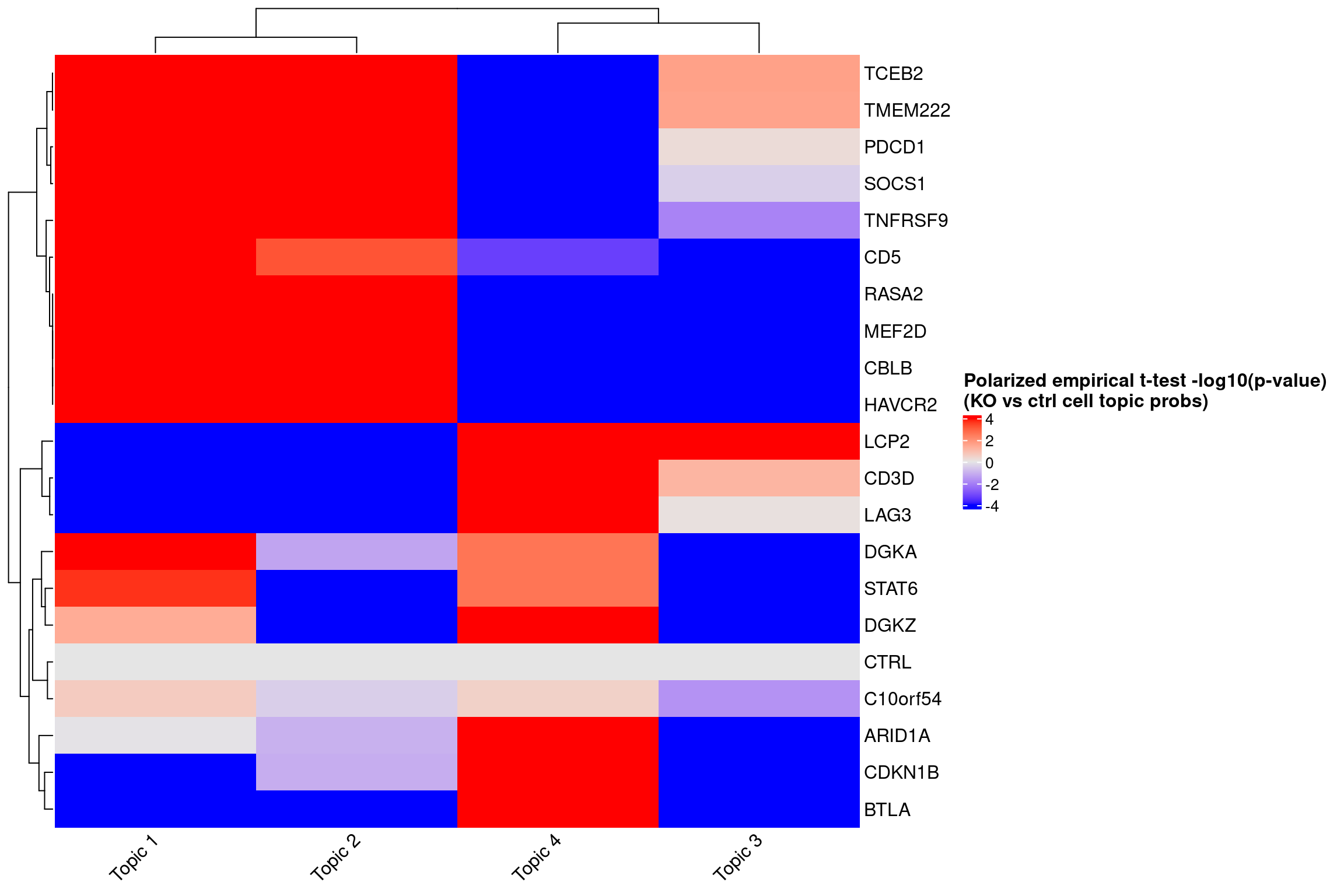
# dev.off()# pdf("music_output/music_merged_4_topics_empirical_tstats_fdr_dotplot.pdf",
# width = 12, height = 8)
KO_names <- rownames(fdr_mat)
dotplot_effectsize(t(effect_mat), t(fdr_mat),
reorder_markers = c(KO_names[KO_names!="CTRL"], "CTRL"),
color_lgd_title = "MUSIC T statistics",
size_lgd_title = "FDR",
max_score = 20,
min_score = -20,
by_score = 10) +
coord_flip() +
theme(axis.text.x = element_text(angle = 45, vjust = 1))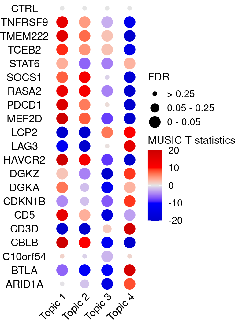
# dev.off()KO_names <- rownames(bonferroni_mat)
dotplot_effectsize(t(effect_mat), t(bonferroni_mat),
reorder_markers = c(KO_names[KO_names!="CTRL"], "CTRL"),
color_lgd_title = "MUSIC T statistics",
size_lgd_title = "Bonferroni\nadjusted p-value",
max_score = 20,
min_score = -20,
by_score = 10) +
coord_flip() +
theme(axis.text.x = element_text(angle = 45, vjust = 1))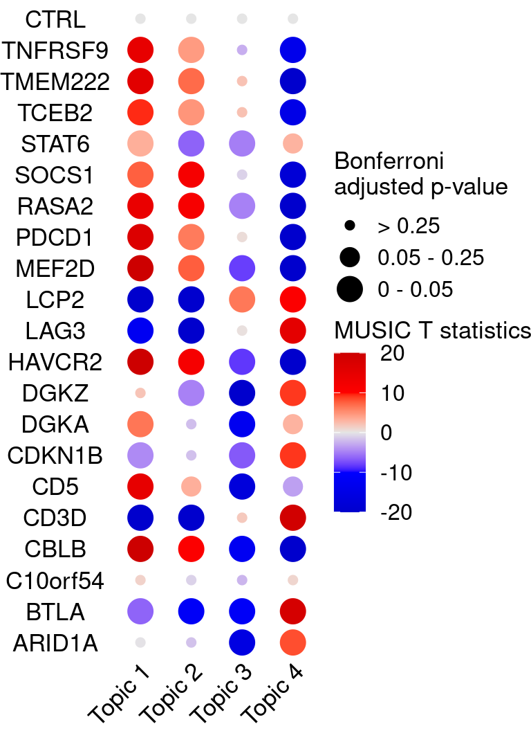
sessionInfo()R version 4.2.0 (2022-04-22)
Platform: x86_64-pc-linux-gnu (64-bit)
Running under: CentOS Linux 7 (Core)
Matrix products: default
BLAS/LAPACK: /software/openblas-0.3.13-el7-x86_64/lib/libopenblas_haswellp-r0.3.13.so
locale:
[1] LC_CTYPE=en_US.UTF-8 LC_NUMERIC=C LC_TIME=C
[4] LC_COLLATE=C LC_MONETARY=C LC_MESSAGES=C
[7] LC_PAPER=C LC_NAME=C LC_ADDRESS=C
[10] LC_TELEPHONE=C LC_MEASUREMENT=C LC_IDENTIFICATION=C
attached base packages:
[1] grid stats4 stats graphics grDevices utils datasets
[8] methods base
other attached packages:
[1] igraph_1.3.4 reshape2_1.4.4 gplots_3.1.3
[4] dplyr_1.0.9 lattice_0.20-45 ggplot2_3.3.6
[7] ComplexHeatmap_2.12.0 MUSIC_1.0 SAVER_1.1.3
[10] clusterProfiler_4.4.4 hash_2.2.6.2 topicmodels_0.2-12
[13] Biostrings_2.64.0 GenomeInfoDb_1.32.2 XVector_0.36.0
[16] IRanges_2.30.0 S4Vectors_0.34.0 BiocGenerics_0.42.0
[19] sp_1.4-7 SeuratObject_4.1.0 Seurat_4.1.1
[22] data.table_1.14.2 workflowr_1.7.0
loaded via a namespace (and not attached):
[1] utf8_1.2.2 reticulate_1.24 tidyselect_1.1.2
[4] RSQLite_2.2.14 AnnotationDbi_1.58.0 htmlwidgets_1.5.4
[7] BiocParallel_1.30.3 Rtsne_0.16 scatterpie_0.1.8
[10] munsell_0.5.0 codetools_0.2-18 ica_1.0-2
[13] future_1.25.0 miniUI_0.1.1.1 withr_2.5.0
[16] spatstat.random_2.2-0 colorspace_2.0-3 GOSemSim_2.22.0
[19] progressr_0.10.0 Biobase_2.56.0 highr_0.9
[22] NLP_0.2-1 knitr_1.39 rstudioapi_0.13
[25] ROCR_1.0-11 tensor_1.5 DOSE_3.22.1
[28] listenv_0.8.0 git2r_0.30.1 slam_0.1-50
[31] GenomeInfoDbData_1.2.8 polyclip_1.10-0 farver_2.1.0
[34] bit64_4.0.5 rprojroot_2.0.3 downloader_0.4
[37] treeio_1.20.2 parallelly_1.31.1 vctrs_0.4.1
[40] generics_0.1.2 xfun_0.30 doParallel_1.0.17
[43] R6_2.5.1 clue_0.3-61 graphlayouts_0.8.1
[46] gridGraphics_0.5-1 bitops_1.0-7 spatstat.utils_2.3-1
[49] cachem_1.0.6 fgsea_1.22.0 assertthat_0.2.1
[52] promises_1.2.0.1 scales_1.2.0 ggraph_2.0.6
[55] enrichplot_1.16.2 rgeos_0.5-9 gtable_0.3.0
[58] Cairo_1.6-0 globals_0.15.0 processx_3.5.3
[61] goftest_1.2-3 tidygraph_1.2.2 rlang_1.0.2
[64] GlobalOptions_0.1.2 splines_4.2.0 lazyeval_0.2.2
[67] spatstat.geom_2.4-0 yaml_2.3.5 abind_1.4-5
[70] httpuv_1.6.5 qvalue_2.28.0 tools_4.2.0
[73] ggplotify_0.1.0 ellipsis_0.3.2 spatstat.core_2.4-2
[76] jquerylib_0.1.4 RColorBrewer_1.1-3 ggridges_0.5.3
[79] Rcpp_1.0.8.3 plyr_1.8.7 zlibbioc_1.42.0
[82] purrr_0.3.4 RCurl_1.98-1.7 ps_1.7.0
[85] rpart_4.1.16 deldir_1.0-6 GetoptLong_1.0.5
[88] viridis_0.6.2 pbapply_1.5-0 cowplot_1.1.1
[91] zoo_1.8-10 ggrepel_0.9.1 cluster_2.1.3
[94] fs_1.5.2 magrittr_2.0.3 scattermore_0.8
[97] DO.db_2.9 circlize_0.4.15 lmtest_0.9-40
[100] RANN_2.6.1 whisker_0.4 fitdistrplus_1.1-8
[103] matrixStats_0.62.0 patchwork_1.1.1 mime_0.12
[106] evaluate_0.15 xtable_1.8-4 shape_1.4.6
[109] gridExtra_2.3 compiler_4.2.0 tibble_3.1.7
[112] shadowtext_0.1.2 KernSmooth_2.23-20 crayon_1.5.1
[115] htmltools_0.5.2 ggfun_0.0.7 mgcv_1.8-40
[118] later_1.3.0 aplot_0.1.7 tidyr_1.2.0
[121] DBI_1.1.3 tweenr_1.0.2 MASS_7.3-56
[124] Matrix_1.4-1 cli_3.3.0 parallel_4.2.0
[127] pkgconfig_2.0.3 getPass_0.2-2 plotly_4.10.0
[130] spatstat.sparse_2.1-1 foreach_1.5.2 xml2_1.3.3
[133] ggtree_3.4.2 bslib_0.3.1 yulab.utils_0.0.5
[136] stringr_1.4.0 callr_3.7.0 digest_0.6.29
[139] sctransform_0.3.3 RcppAnnoy_0.0.19 spatstat.data_2.2-0
[142] tm_0.7-8 rmarkdown_2.14 leiden_0.4.2
[145] fastmatch_1.1-3 tidytree_0.4.0 uwot_0.1.11
[148] gtools_3.9.2 shiny_1.7.1 modeltools_0.2-23
[151] rjson_0.2.21 lifecycle_1.0.1 nlme_3.1-157
[154] jsonlite_1.8.0 viridisLite_0.4.0 fansi_1.0.3
[157] pillar_1.7.0 KEGGREST_1.36.2 fastmap_1.1.0
[160] httr_1.4.3 survival_3.3-1 GO.db_3.15.0
[163] glue_1.6.2 iterators_1.0.14 png_0.1-7
[166] bit_4.0.4 ggforce_0.3.4 stringi_1.7.6
[169] sass_0.4.1 blob_1.2.3 caTools_1.18.2
[172] memoise_2.0.1 ape_5.6-2 irlba_2.3.5
[175] future.apply_1.9.0