MUSIC analysis on LUHMES CROP-seq data
Kaixuan Luo
2022-07-14
Last updated: 2022-09-20
Checks: 7 0
Knit directory: GSFA_analysis/
This reproducible R Markdown analysis was created with workflowr (version 1.7.0). The Checks tab describes the reproducibility checks that were applied when the results were created. The Past versions tab lists the development history.
Great! Since the R Markdown file has been committed to the Git repository, you know the exact version of the code that produced these results.
Great job! The global environment was empty. Objects defined in the global environment can affect the analysis in your R Markdown file in unknown ways. For reproduciblity it’s best to always run the code in an empty environment.
The command set.seed(20220524) was run prior to running
the code in the R Markdown file. Setting a seed ensures that any results
that rely on randomness, e.g. subsampling or permutations, are
reproducible.
Great job! Recording the operating system, R version, and package versions is critical for reproducibility.
Nice! There were no cached chunks for this analysis, so you can be confident that you successfully produced the results during this run.
Great job! Using relative paths to the files within your workflowr project makes it easier to run your code on other machines.
Great! You are using Git for version control. Tracking code development and connecting the code version to the results is critical for reproducibility.
The results in this page were generated with repository version a8e275a. See the Past versions tab to see a history of the changes made to the R Markdown and HTML files.
Note that you need to be careful to ensure that all relevant files for
the analysis have been committed to Git prior to generating the results
(you can use wflow_publish or
wflow_git_commit). workflowr only checks the R Markdown
file, but you know if there are other scripts or data files that it
depends on. Below is the status of the Git repository when the results
were generated:
Ignored files:
    Ignored:    .DS_Store
    Ignored:    .Rhistory
    Ignored:    .Rproj.user/

Untracked files:
    Untracked:  Rplots.pdf
    Untracked:  analysis/check_Tcells_datasets.Rmd
    Untracked:  analysis/fscLVM_analysis.Rmd
    Untracked:  analysis/spca_LUHMES_data.Rmd
    Untracked:  analysis/test_seurat.Rmd
    Untracked:  code/gsfa_negctrl_job.sbatch
    Untracked:  code/music_LUHMES_Yifan.R
    Untracked:  code/plotting_functions.R
    Untracked:  code/run_fscLVM_LUHMES_data.R
    Untracked:  code/run_gsfa_2groups_negctrl.R
    Untracked:  code/run_gsfa_negctrl.R
    Untracked:  code/run_music_LUHMES.R
    Untracked:  code/run_music_LUHMES_data.sbatch
    Untracked:  code/run_music_LUHMES_data_20topics.R
    Untracked:  code/run_music_LUHMES_data_20topics.sbatch
    Untracked:  code/run_sceptre_Tcells_data.sbatch
    Untracked:  code/run_sceptre_Tcells_stimulated_data.sbatch
    Untracked:  code/run_sceptre_Tcells_test_data.sbatch
    Untracked:  code/run_sceptre_Tcells_unstimulated_data.sbatch
    Untracked:  code/run_sceptre_permuted_data.sbatch
    Untracked:  code/run_spca_LUHMES.R
    Untracked:  code/run_spca_TCells.R
    Untracked:  code/run_twostep_clustering_LUHMES_data.sbatch
    Untracked:  code/run_twostep_clustering_Tcells_data.sbatch
    Untracked:  code/run_unguided_gsfa_LUHMES.R
    Untracked:  code/run_unguided_gsfa_LUHMES.sbatch
    Untracked:  code/run_unguided_gsfa_Tcells.R
    Untracked:  code/run_unguided_gsfa_Tcells.sbatch
    Untracked:  code/sceptre_LUHMES_data.R
    Untracked:  code/sceptre_Tcells_stimulated_data.R
    Untracked:  code/sceptre_Tcells_unstimulated_data.R
    Untracked:  code/sceptre_permutation_analysis.R
    Untracked:  code/sceptre_permute_analysis.R
    Untracked:  code/seurat_sim_fpr_tpr.R
    Untracked:  code/unguided_GFSA_mixture_normal_prior.cpp

Unstaged changes:
    Modified:   analysis/sceptre_TCells_data.Rmd
    Modified:   analysis/twostep_clustering_LUHMES_data.Rmd
    Modified:   code/run_sceptre_LUHMES_data.R
    Modified:   code/run_sceptre_LUHMES_data.sbatch
    Modified:   code/run_sceptre_LUHMES_permuted_data.R
    Modified:   code/run_sceptre_Tcells_permuted_data.R
    Modified:   code/run_sceptre_cropseq_data.sbatch
    Modified:   code/run_twostep_clustering_LUHMES_data.R
    Modified:   code/sceptre_analysis.R
Note that any generated files, e.g. HTML, png, CSS, etc., are not included in this status report because it is ok for generated content to have uncommitted changes.
These are the previous versions of the repository in which changes were
made to the R Markdown (analysis/music_LUHMES_data.Rmd) and
HTML (docs/music_LUHMES_data.html) files. If you’ve
configured a remote Git repository (see ?wflow_git_remote),
click on the hyperlinks in the table below to view the files as they
were in that past version.
| File | Version | Author | Date | Message |
|---|---|---|---|---|
| Rmd | a8e275a | kevinlkx | 2022-09-20 | updated dot plots |
| html | 31d48d1 | kevinlkx | 2022-09-20 | Build site. |
| Rmd | f02521e | kevinlkx | 2022-09-20 | updated the dot plots and saved as pdf |
| html | df4b0c6 | kevinlkx | 2022-08-11 | Build site. |
| Rmd | b979400 | kevinlkx | 2022-08-11 | fix intro formatting |
| html | a2297e5 | kevinlkx | 2022-08-11 | Build site. |
| Rmd | a0b124f | kevinlkx | 2022-08-11 | added dot plots with Bonferroni adjusted p-value |
| html | 43b3a70 | kevinlkx | 2022-08-01 | Build site. |
| Rmd | 706ef41 | kevinlkx | 2022-08-01 | test 4-6 topics |
| html | e54a27e | kevinlkx | 2022-07-29 | Build site. |
| Rmd | 66afbb0 | kevinlkx | 2022-07-29 | update dotplot figure legend |
| html | 2763f33 | kevinlkx | 2022-07-29 | Build site. |
| Rmd | f5bca8a | kevinlkx | 2022-07-29 | added dotplots with MUSIC empirical TPD FDR |
| html | 223426b | kevinlkx | 2022-07-25 | Build site. |
| Rmd | 3cbce15 | kevinlkx | 2022-07-25 | update music results for LUHMES data |
| html | 5200b77 | kevinlkx | 2022-07-19 | Build site. |
| Rmd | 358270c | kevinlkx | 2022-07-19 | run MUSIC on LUHMES data |
slurm setting
sinteractive --partition=broadwl --account=pi-xinhe --mem=30G --time=10:00:00 --cpus-per-task=10MUSIC website: https://github.com/bm2-lab/MUSIC
Scripts for running the analysis:
cd /project2/xinhe/kevinluo/GSFA/music_analysis/log

sbatch --mem=50G --cpus-per-task=10 ~/projects/GSFA_analysis/code/run_music_LUHMES_data.sbatch
Running time check
cd /project2/xinhe/kevinluo/GSFA/music_analysis/log

sbatch --mem=50G --cpus-per-task=10 ~/projects/GSFA_analysis/code/run_music_LUHMES_data_20topics.sbatch
About the data sets
CROP-seq datasets:
/project2/xinhe/yifan/Factor_analysis/shared_data/. The
data are Seurat objects, with raw gene counts stored in
obj@assays$RNA@counts, and cell meta data stored in
obj@meta.data. Normalized and scaled data used for GSFA are
stored in obj@assays$RNA@scale.data, the rownames of which
are the 6k genes used for GSFA.
Load packages
dyn.load('/software/geos-3.7.0-el7-x86_64/lib64/libgeos_c.so') # attach the geos lib for Seurat
suppressPackageStartupMessages(library(data.table))
suppressPackageStartupMessages(library(Seurat))
suppressPackageStartupMessages(library(MUSIC))
suppressPackageStartupMessages(library(ComplexHeatmap))
suppressPackageStartupMessages(library(ggplot2))
theme_set(theme_bw() + theme(plot.title = element_text(size = 14, hjust = 0.5),
                             axis.title = element_text(size = 14),
                             axis.text = element_text(size = 13),
                             legend.title = element_text(size = 13),
                             legend.text = element_text(size = 12),
                             panel.grid.minor = element_blank())
)

source("code/plotting_functions.R")
functions
## Adapted over MUSIC's Diff_topic_distri() function
Empirical_topic_prob_diff <- function(model, perturb_information,
                                      permNum = 10^4, seed = 1000){
  require(reshape2)
  require(dplyr)
  require(ComplexHeatmap)
  options(warn = -1)
  prob_mat <- model@gamma
  row.names(prob_mat) <- model@documents
  topicNum <- ncol(prob_mat)
  topicName <- paste0('Topic_', 1:topicNum)
  colnames(prob_mat) <- topicName
  ko_name <- unique(perturb_information)
  prob_df <- data.frame(prob_mat,
                        samples = rownames(prob_mat),
                        knockout = perturb_information)

  prob_df <- melt(prob_df, id = c('samples', 'knockout'), variable.name = "topic")

  summary_df <- prob_df %>%
    group_by(knockout, topic) %>%
    summarise(number = sum(value)) %>%
    ungroup() %>%
    group_by(knockout) %>%
    mutate(cellNum = sum(number)) %>%
    ungroup() %>%
    mutate(ratio = number/cellNum)

  summary_df$ctrlNum <- rep(summary_df$cellNum[summary_df$knockout == "CTRL"],
                            length(ko_name))
  summary_df$ctrl_ratio <- rep(summary_df$ratio[summary_df$knockout == "CTRL"],
                               length(ko_name))
  summary_df <- summary_df %>% mutate(diff_index = ratio - ctrl_ratio)

  test_df <- data.frame(matrix(nrow = length(ko_name) * topicNum, ncol = 5))
  colnames(test_df) <- c("knockout", "topic", "obs_t_stats", "obs_pval", "empirical_pval")
  k <- 1
  for(i in topicName){
    prob_df.topic <- prob_df[prob_df$topic == i, ]
    ctrl_topic <- prob_df.topic$value[prob_df.topic$knockout == "CTRL"]
    ctrl_topic_z <- (ctrl_topic - mean(ctrl_topic)) / sqrt(var(ctrl_topic))
    for(j in ko_name){
      ko_topic <- prob_df.topic$value[prob_df.topic$knockout == j]
      ko_topic_z <- (ko_topic - mean(ctrl_topic)) / sqrt(var(ctrl_topic))
      test_df$knockout[k] <- j
      test_df$topic[k] <- i
      test <- t.test(ko_topic_z, ctrl_topic_z)
      test_df$obs_t_stats[k] <- test$statistic
      test_df$obs_pval[k] <- test$p.value
      k <- k + 1
    }
  }

  ## Permutation on the perturbation conditions:
  # permNum <- 10^4
  print(paste0("Performing permutation for ", permNum, " rounds."))
  perm_t_stats <- matrix(0, nrow = nrow(test_df), ncol = permNum)
  set.seed(seed)
  for (perm in 1:permNum){
    perm_prob_df <- data.frame(prob_mat,
                               samples = rownames(prob_mat),
                               knockout = perturb_information[sample(length(perturb_information))])
    perm_prob_df <- melt(perm_prob_df, id = c('samples', 'knockout'), variable.name = "topic")
    k <- 1
    for(i in topicName){
      perm_prob_df.topic <- perm_prob_df[perm_prob_df$topic == i, ]
      ctrl_topic <- perm_prob_df.topic$value[perm_prob_df.topic$knockout == "CTRL"]
      ctrl_topic_z <- (ctrl_topic - mean(ctrl_topic)) / sqrt(var(ctrl_topic))
      for(j in ko_name){
        ko_topic <- perm_prob_df.topic$value[perm_prob_df.topic$knockout == j]
        ko_topic_z <- (ko_topic - mean(ctrl_topic)) / sqrt(var(ctrl_topic))
        test <- t.test(ko_topic_z, ctrl_topic_z)
        perm_t_stats[k, perm] <- test$statistic
        k <- k + 1
      }
    }
    if (perm %% 1000 == 0){
      print(paste0(perm, " rounds finished."))
    }
  }
  ## Compute two-sided empirical p value:
  for (k in 1:nrow(test_df)){
    test_df$empirical_pval[k] <-
      2 * min(mean(perm_t_stats[k, ] <= test_df$obs_t_stats[k]),
              mean(perm_t_stats[k, ] >= test_df$obs_t_stats[k]))
  }
  test_df <- test_df %>%
    mutate(empirical_pval = ifelse(empirical_pval == 0, 1/permNum, empirical_pval)) %>%
    mutate(empirical_pval = ifelse(empirical_pval > 1, 1, empirical_pval))

  summary_df <- inner_join(summary_df, test_df, by = c("knockout", "topic"))
  summary_df <- summary_df %>%
    mutate(polar_log10_pval = ifelse(obs_t_stats > 0, -log10(empirical_pval), log10(empirical_pval)))
  return(summary_df)
}
Set directories
data_dir <- "/project2/xinhe/yifan/Factor_analysis/LUHMES/"
res_dir <- "/project2/xinhe/kevinluo/GSFA/music_analysis/LUHMES"
dir.create(file.path(res_dir,"/music_output"), recursive = TRUE, showWarnings = FALSE)setwd(res_dir)Run MUSIC
0. Load input data
feature.names <- data.frame(fread(paste0(data_dir, "GSE142078_raw/GSM4219575_Run1_genes.tsv.gz"),
                                  header = FALSE), stringsAsFactors = FALSE)

# combined_obj <- readRDS("processed_data/seurat_obj.merged_scaled_detect_01.corrected_new.rds")
combined_obj <- readRDS("/project2/xinhe/yifan/Factor_analysis/shared_data/LUHMES_cropseq_data_seurat.rds")
expression_profile <- combined_obj@assays$RNA@counts
rownames(expression_profile) <- feature.names$V2[match(rownames(expression_profile),
                                                       feature.names$V1)]

cat("Dimension of expression profile matrix: \n")
dim(expression_profile)

targets <- names(combined_obj@meta.data)[4:18]
targets[targets == "Nontargeting"] <- "CTRL"
cat("Targets: \n")
print(targets)

perturb_information <- apply(combined_obj@meta.data[4:18], 1,
                             function(x){ targets[which(x > 0)] })
Dimension of expression profile matrix:
[1] 33694 8708
Targets:
[1] "ADNP" "ARID1B" "ASH1L" "CHD2" "CHD8" "CTNND2" "DYRK1A" "HDAC5"
[9] "MECP2" "MYT1L" "CTRL" "POGZ" "PTEN" "RELN" "SETD5" 1. Data preprocessing
crop_seq_list <- Input_preprocess(expression_profile, perturb_information)

crop_seq_qc <- Cell_qc(crop_seq_list$expression_profile,
                       crop_seq_list$perturb_information,
                       species = "Hs", plot = F)

crop_seq_imputation <- Data_imputation(crop_seq_qc$expression_profile,
                                       crop_seq_qc$perturb_information,
                                       cpu_num = 10)
saveRDS(crop_seq_imputation, "music_output/music_imputation.merged.rds")

crop_seq_filtered <- Cell_filtering(crop_seq_imputation$expression_profile,
                                    crop_seq_imputation$perturb_information,
                                    cpu_num = 10)
saveRDS(crop_seq_filtered, "music_output/music_filtered.merged.rds")
2. Model building
Obtain highly dispersion differentially expressed genes.
crop_seq_filtered <- readRDS("music_output/music_filtered.merged.rds")
dim(crop_seq_filtered$expression_profile)
length(crop_seq_filtered$perturb_information)

crop_seq_vargene <- Get_high_varGenes(crop_seq_filtered$expression_profile,
                                      crop_seq_filtered$perturb_information, plot = T)
saveRDS(crop_seq_vargene, "music_output/music_vargene.merged.rds")

crop_seq_vargene <- readRDS("music_output/music_vargene.merged.rds")
dim(crop_seq_vargene$expression_profile)

crop_seq_vargene$expression_profile[1:5,1:5]
length(crop_seq_vargene$perturb_information)
get topics.
## Get_topics() can take up to a few hours to finish,
## depending on the size of data
system.time(
  topic_1 <- Get_topics(crop_seq_vargene$expression_profile,
                        crop_seq_vargene$perturb_information,
                        topic_number = 5))
saveRDS(topic_1, "music_output/music_merged_5_topics.rds")

system.time(
  topic_2 <- Get_topics(crop_seq_vargene$expression_profile,
                        crop_seq_vargene$perturb_information,
                        topic_number = 10))
saveRDS(topic_2, "music_output/music_merged_10_topics.rds")

system.time(
  topic_3 <- Get_topics(crop_seq_vargene$expression_profile,
                        crop_seq_vargene$perturb_information,
                        topic_number = 15))
saveRDS(topic_3, "music_output/music_merged_15_topics.rds")

system.time(
  topic_4 <- Get_topics(crop_seq_vargene$expression_profile,
                        crop_seq_vargene$perturb_information,
                        topic_number = 20))
saveRDS(topic_4, "music_output/music_merged_20_topics.rds")

## try fewer numbers of topics
system.time(
  topic_5 <- Get_topics(crop_seq_vargene$expression_profile,
                        crop_seq_vargene$perturb_information,
                        topic_number = 4))
saveRDS(topic_5, "music_output/music_merged_4_topics.rds")

system.time(
  topic_6 <- Get_topics(crop_seq_vargene$expression_profile,
                        crop_seq_vargene$perturb_information,
                        topic_number = 6))
saveRDS(topic_6, "music_output/music_merged_6_topics.rds")
3. Pick the number of topics
topic_1 <- readRDS("music_output/music_merged_4_topics.rds")
topic_2 <- readRDS("music_output/music_merged_5_topics.rds")
topic_3 <- readRDS("music_output/music_merged_6_topics.rds")
topic_4 <- readRDS("music_output/music_merged_10_topics.rds")
topic_5 <- readRDS("music_output/music_merged_15_topics.rds")
topic_6 <- readRDS("music_output/music_merged_20_topics.rds")

topic_model_list <- list()
topic_model_list$models <- list()
topic_model_list$perturb_information <- topic_1$perturb_information
topic_model_list$models[[1]] <- topic_1$models[[1]]
topic_model_list$models[[2]] <- topic_2$models[[1]]
topic_model_list$models[[3]] <- topic_3$models[[1]]
topic_model_list$models[[4]] <- topic_4$models[[1]]
topic_model_list$models[[5]] <- topic_5$models[[1]]
topic_model_list$models[[6]] <- topic_6$models[[1]]

optimalModel <- Select_topic_number(topic_model_list$models,
                                    plot = T,
                                    plot_path = "music_output/select_topic_number_4to6to20.pdf")
Summarize the results
Summarize the results under 20 topics to be comparable to GSFA
Gene ontology annotations for top topics
topic_res <- readRDS("music_output/music_merged_20_topics.rds")

topic_func <- Topic_func_anno(topic_res$models[[1]], species = "Hs")
saveRDS(topic_func, "music_output/topic_func.rds")
topic_func <- readRDS("music_output/topic_func.rds")
# pdf("music_output/music_merged_20_topics_GO_annotations.pdf",
# width = 14, height = 12)
ggplot(topic_func$topic_annotation_result) +
geom_point(aes(x = Cluster, y = Description,
size = Count, color = -log10(qvalue))) +
scale_color_gradientn(colors = c("blue", "red")) +
theme_bw() +
theme(axis.title = element_blank(),
axis.text.x = element_text(angle = 45, hjust = 1))
# dev.off()Perturbation effect prioritizing
# calculate topic distribution for each cell.
distri_diff <- Diff_topic_distri(topic_res$models[[1]],
                                 topic_res$perturb_information,
                                 plot = T)
saveRDS(distri_diff, "music_output/distri_diff.rds")

distri_diff <- readRDS("music_output/distri_diff.rds")
t_D_diff_matrix <- dcast(distri_diff %>% dplyr::select(knockout, variable, t_D_diff),
                         knockout ~ variable)
rownames(t_D_diff_matrix) <- t_D_diff_matrix$knockout
t_D_diff_matrix$knockout <- NULL
# pdf("music_output/music_merged_20_topics_TPD_heatmap.pdf", width = 12, height = 8)
Heatmap(t_D_diff_matrix,
name = "Topic probability difference (vs ctrl)",
cluster_rows = T, cluster_columns = T,
column_names_rot = 45,
heatmap_legend_param = list(title_gp = gpar(fontsize = 12, fontface = "bold")))
# dev.off()Overall perturbation effect ranking list.
distri_diff <- readRDS(file.path(res_dir, "music_output/distri_diff.rds"))

rank_overall_result <- Rank_overall(distri_diff)
print(rank_overall_result)
# saveRDS(rank_overall_result, "music_output/rank_overall_result.rds")
perturbation ranking Score off_target
1 ASH1L 1 85.91013 none
2 SETD5 2 79.56861 none
3 ARID1B 3 77.59034 none
4 CHD8 4 70.16751 none
5 PTEN 5 66.48328 none
6 POGZ 6 64.12727 none
7 MECP2 7 62.10662 none
8 RELN 8 59.26017 none
9 CHD2 9 55.85265 none
10 MYT1L 10 39.67237 none
11 ADNP 11 39.06289 none
12 DYRK1A 12 38.98911 none
13 HDAC5 13 38.48395 nonetopic-specific ranking list.
rank_topic_specific_result <- Rank_specific(distri_diff)
head(rank_topic_specific_result, 10)
# saveRDS(rank_topic_specific_result, "music_output/rank_topic_specific_result.rds")
topic perturbation ranking
1 Topic1 ARID1B 1
2 Topic1 CHD8 2
3 Topic1 SETD5 3
4 Topic1 MECP2 4
5 Topic1 POGZ 5
6 Topic1 PTEN 6
7 Topic1 HDAC5 7
8 Topic1 DYRK1A 8
9 Topic1 ADNP 9
10 Topic1 RELN 10Perturbation correlation.
perturb_cor <- Correlation_perturbation(distri_diff,
                                        cutoff = 0.5, gene = "all", plot = T,
                                        plot_path = file.path(res_dir, "music_output/correlation_network_20_topics.pdf"))

head(perturb_cor, 10)
# saveRDS(perturb_cor, "music_output/perturb_cor.rds")
Perturbation_1 Perturbation_2 Correlation
2 ARID1B ADNP -0.36642339
3 ASH1L ADNP 0.60467107
16 ASH1L ARID1B 0.12772609
30 CHD2 ASH1L 0.91852307
4 CHD2 ADNP 0.81036468
17 CHD2 ARID1B 0.03762586
18 CHD8 ARID1B 0.89232727
5 CHD8 ADNP -0.26907399
31 CHD8 ASH1L 0.25264119
44 CHD8 CHD2 0.13836576Adaptation to the code to generate calibrated empirical TPD scores
summary_df <- Empirical_topic_prob_diff(topic_res$models[[1]],
                                        topic_res$perturb_information)
saveRDS(summary_df, "music_output/music_merged_20_topics_ttest_summary.rds")
summary_df <- readRDS(file.path(res_dir, "music_output/music_merged_20_topics_ttest_summary.rds"))
summary_df$topic <- gsub("_", " ", summary_df$topic)
summary_df$topic <- factor(summary_df$topic, levels = paste("Topic", 1:length(unique(summary_df$topic))))
summary_df$fdr <- p.adjust(summary_df$empirical_pval, method = "BH")
summary_df$bonferroni_adj <- p.adjust(summary_df$empirical_pval, method = "bonferroni")
log10_pval_mat <- dcast(summary_df %>% dplyr::select(knockout, topic, polar_log10_pval),
knockout ~ topic)
rownames(log10_pval_mat) <- log10_pval_mat$knockout
log10_pval_mat$knockout <- NULL
effect_mat <- dcast(summary_df %>% dplyr::select(knockout, topic, obs_t_stats), knockout ~ topic)
rownames(effect_mat) <- effect_mat$knockout
effect_mat$knockout <- NULL
fdr_mat <- dcast(summary_df %>% dplyr::select(knockout, topic, fdr), knockout ~ topic)
rownames(fdr_mat) <- fdr_mat$knockout
fdr_mat$knockout <- NULL
bonferroni_mat <- dcast(summary_df %>% dplyr::select(knockout, topic, bonferroni_adj), knockout ~ topic)
rownames(bonferroni_mat) <- bonferroni_mat$knockout
bonferroni_mat$knockout <- NULL# pdf("music_output/music_merged_20_topics_empirical_tstats_heatmap.pdf",
# width = 12, height = 8)
ht <- Heatmap(log10_pval_mat,
name = "Polarized empirical t-test -log10(p-value)\n(KO vs ctrl cell topic probs)",
col = circlize::colorRamp2(breaks = c(-4, 0, 4), colors = c("blue", "grey90", "red")),
cluster_rows = T, cluster_columns = T,
column_names_rot = 45,
heatmap_legend_param = list(title_gp = gpar(fontsize = 12,
fontface = "bold")))
draw(ht)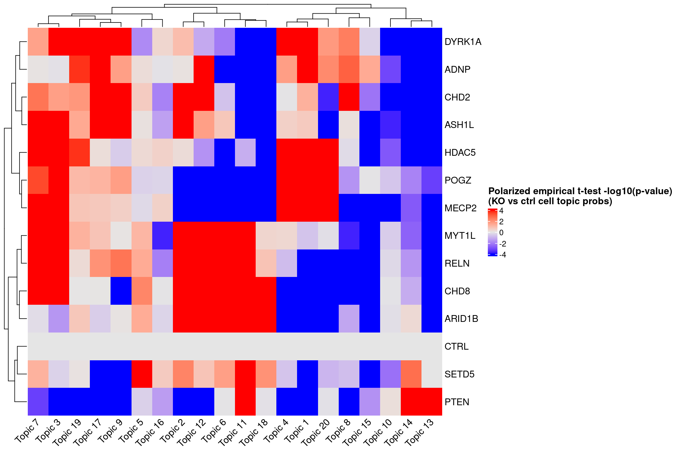
# dev.off()# pdf("music_output/music_merged_20_topics_empirical_tstats_fdr_dotplot.pdf",
# width = 12, height = 8)
KO_names <- rownames(fdr_mat)
dotplot_effectsize(t(effect_mat), t(fdr_mat),
reorder_markers = c(KO_names[KO_names!="CTRL"], "CTRL"),
color_lgd_title = "MUSIC T statistics",
size_lgd_title = "FDR",
max_score = 20,
min_score = -20,
by_score = 10) +
coord_flip() +
theme(axis.text.x = element_text(angle = 45, vjust = 1))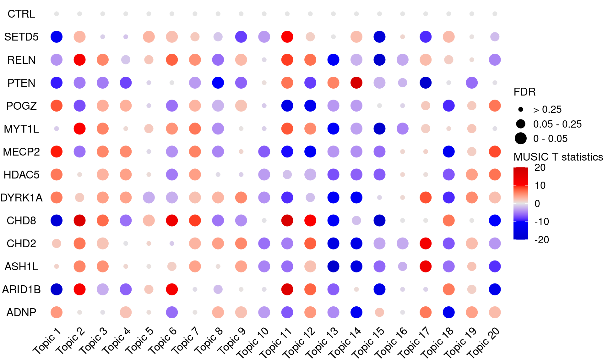
# dev.off()KO_names <- rownames(bonferroni_mat)
dotplot_effectsize(t(effect_mat), t(bonferroni_mat),
reorder_markers = c(KO_names[KO_names!="CTRL"], "CTRL"),
color_lgd_title = "MUSIC T statistics",
size_lgd_title = "Bonferroni\nadjusted p-value",
max_score = 20,
min_score = -20,
by_score = 10) +
coord_flip() +
theme(axis.text.x = element_text(angle = 45, vjust = 1))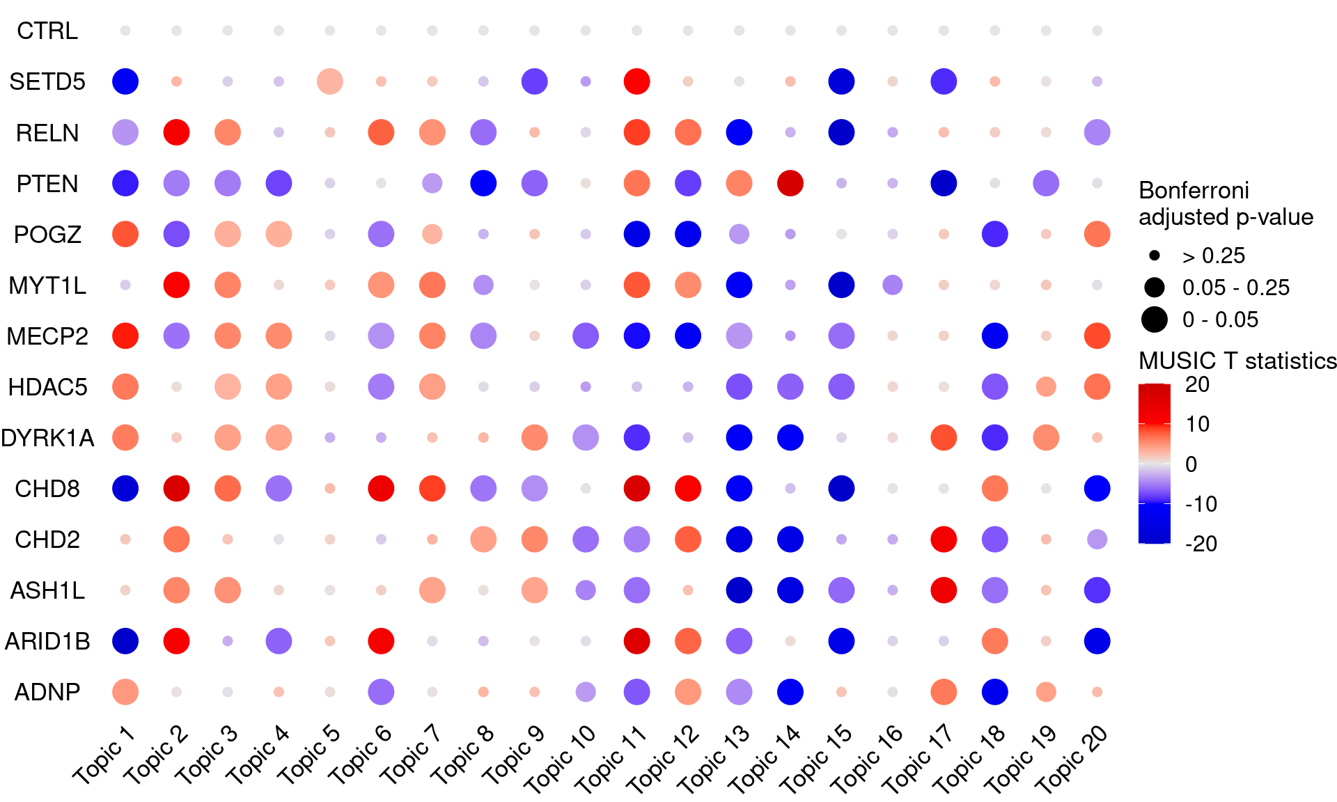
Summarize the results using the optimal number of topics selected by the score
Pick optimal number of topics
topic_1 <- readRDS("music_output/music_merged_4_topics.rds")
topic_2 <- readRDS("music_output/music_merged_5_topics.rds")
topic_3 <- readRDS("music_output/music_merged_6_topics.rds")

topic_model_list <- list()
topic_model_list$models <- list()
topic_model_list$perturb_information <- topic_1$perturb_information
topic_model_list$models[[1]] <- topic_1$models[[1]]
topic_model_list$models[[2]] <- topic_2$models[[1]]
topic_model_list$models[[3]] <- topic_3$models[[1]]

optimalModel <- Select_topic_number(topic_model_list$models,
                                    plot = T,
                                    plot_path = "music_output/select_topic_number_4to6.pdf")

optimalModel
saveRDS(optimalModel, "music_output/optimalModel_4_topics.rds")
Gene ontology annotations for top topics
topic_func <- Topic_func_anno(optimalModel, species = "Hs", plot_path = "music_output/topic_annotation_GO_4_topics.pdf")
saveRDS(topic_func, "music_output/topic_func_4_topics.rds")
topic_func <- readRDS("music_output/topic_func_4_topics.rds")
pdf("music_output/music_merged_4_topics_GO_annotations.pdf",
width = 14, height = 12)
ggplot(topic_func$topic_annotation_result) +
geom_point(aes(x = Cluster, y = Description,
size = Count, color = -log10(qvalue))) +
scale_color_gradientn(colors = c("blue", "red")) +
theme_bw() +
theme(axis.title = element_blank(),
axis.text.x = element_text(angle = 45, hjust = 1))
dev.off()Perturbation effect prioritizing
# calculate topic distribution for each cell.
distri_diff <- Diff_topic_distri(optimalModel,
                                 topic_model_list$perturb_information,
                                 plot = T,
                                 plot_path = "music_output/distribution_of_topic_4_topics.pdf")
saveRDS(distri_diff, "music_output/distri_diff_4_topics.rds")

t_D_diff_matrix <- dcast(distri_diff %>% dplyr::select(knockout, variable, t_D_diff),
                         knockout ~ variable)
rownames(t_D_diff_matrix) <- t_D_diff_matrix$knockout
t_D_diff_matrix$knockout <- NULL
pdf("music_output/music_merged_4_topics_TPD_heatmap.pdf", width = 12, height = 8)
Heatmap(t_D_diff_matrix,
name = "Topic probability difference (vs ctrl)",
cluster_rows = T, cluster_columns = T,
column_names_rot = 45,
heatmap_legend_param = list(title_gp = gpar(fontsize = 12, fontface = "bold")))
dev.off()The overall perturbation effect ranking list.
distri_diff <- readRDS(file.path(res_dir, "music_output/distri_diff_4_topics.rds"))

rank_overall_result <- Rank_overall(distri_diff)
print(rank_overall_result)
# saveRDS(rank_overall_result, "music_output/rank_overall_4_topics_result.rds")
perturbation ranking Score off_target
1 SETD5 1 32.265899 none
2 CHD8 2 29.938862 none
3 ASH1L 3 27.619199 none
4 ARID1B 4 26.301156 none
5 PTEN 5 21.192816 none
6 RELN 6 19.653807 none
7 POGZ 7 18.954187 none
8 MECP2 8 15.761953 none
9 CHD2 9 15.395937 none
10 MYT1L 10 13.622441 none
11 DYRK1A 11 11.767298 none
12 HDAC5 12 9.232891 none
13 ADNP 13 8.549708 noneTopic-specific ranking list.
rank_topic_specific_result <- Rank_specific(distri_diff)
print(rank_topic_specific_result)
# saveRDS(rank_topic_specific_result, "music_output/rank_topic_specific_4_topics_result.rds")
topic perturbation ranking
1 Topic1 ARID1B 1
2 Topic1 CHD8 2
3 Topic1 POGZ 3
4 Topic1 MECP2 4
5 Topic2 MECP2 1
6 Topic2 MYT1L 2
7 Topic2 HDAC5 3
8 Topic2 RELN 4
9 Topic2 ASH1L 5
10 Topic2 CHD8 6
11 Topic2 PTEN 7
12 Topic2 POGZ 8
13 Topic2 DYRK1A 9
14 Topic2 CHD2 10
15 Topic2 ARID1B 11
16 Topic2 SETD5 12
17 Topic3 ASH1L 1
18 Topic3 CHD2 2
19 Topic3 PTEN 3
20 Topic3 DYRK1A 4
21 Topic3 ADNP 5
22 Topic3 HDAC5 6
23 Topic3 POGZ 7
24 Topic3 SETD5 8
25 Topic3 MECP2 9
26 Topic3 MYT1L 10
27 Topic3 RELN 11
28 Topic4 SETD5 1
29 Topic4 CHD8 2
30 Topic4 ARID1B 3
31 Topic4 RELN 4
32 Topic4 ADNP 5
33 Topic4 MYT1L 6
34 Topic4 PTEN 7
35 Topic4 POGZ 8
36 Topic4 DYRK1A 9
37 Topic4 MECP2 10
38 Topic4 HDAC5 11Perturbation correlation.
perturb_cor <- Correlation_perturbation(distri_diff,
                                        cutoff = 0.5, gene = "all", plot = T,
                                        plot_path = file.path(res_dir, "music_output/correlation_network_4_topics.pdf"))

head(perturb_cor, 10)
# saveRDS(perturb_cor, "music_output/perturb_cor_4_topics.rds")
Perturbation_1 Perturbation_2 Correlation
2 ARID1B ADNP -0.46218365
3 ASH1L ADNP 0.80478083
16 ASH1L ARID1B 0.10678869
30 CHD2 ASH1L 0.99394160
4 CHD2 ADNP 0.83311135
17 CHD2 ARID1B 0.08935393
18 CHD8 ARID1B 0.98008439
5 CHD8 ADNP -0.51737973
31 CHD8 ASH1L 0.08031335
44 CHD8 CHD2 0.04192687Adaptation to the code to generate calibrated empirical TPD scores
summary_df <- Empirical_topic_prob_diff(optimalModel,
                                        topic_model_list$perturb_information)
saveRDS(summary_df, "music_output/music_merged_4_topics_ttest_summary.rds")
summary_df <- readRDS(file.path(res_dir, "music_output/music_merged_4_topics_ttest_summary.rds"))
summary_df$topic <- gsub("_", " ", summary_df$topic)
summary_df$topic <- factor(summary_df$topic, levels = paste("Topic", 1:length(unique(summary_df$topic))))
summary_df$fdr <- p.adjust(summary_df$empirical_pval, method = "BH")
summary_df$bonferroni_adj <- p.adjust(summary_df$empirical_pval, method = "bonferroni")
log10_pval_mat <- dcast(summary_df %>% dplyr::select(knockout, topic, polar_log10_pval),
knockout ~ topic)
rownames(log10_pval_mat) <- log10_pval_mat$knockout
log10_pval_mat$knockout <- NULL
effect_mat <- dcast(summary_df %>% dplyr::select(knockout, topic, obs_t_stats), knockout ~ topic)
rownames(effect_mat) <- effect_mat$knockout
effect_mat$knockout <- NULL
fdr_mat <- dcast(summary_df %>% dplyr::select(knockout, topic, fdr), knockout ~ topic)
rownames(fdr_mat) <- fdr_mat$knockout
fdr_mat$knockout <- NULL
bonferroni_mat <- dcast(summary_df %>% dplyr::select(knockout, topic, bonferroni_adj), knockout ~ topic)
rownames(bonferroni_mat) <- bonferroni_mat$knockout
bonferroni_mat$knockout <- NULL# pdf("music_output/music_merged_4_topics_empirical_tstats_heatmap.pdf",
# width = 12, height = 8)
ht <- Heatmap(log10_pval_mat,
name = "Polarized empirical t-test -log10(p-value)\n(KO vs ctrl cell topic probs)",
col = circlize::colorRamp2(breaks = c(-4, 0, 4), colors = c("blue", "grey90", "red")),
cluster_rows = T, cluster_columns = T,
column_names_rot = 45,
heatmap_legend_param = list(title_gp = gpar(fontsize = 12,
fontface = "bold")))
draw(ht)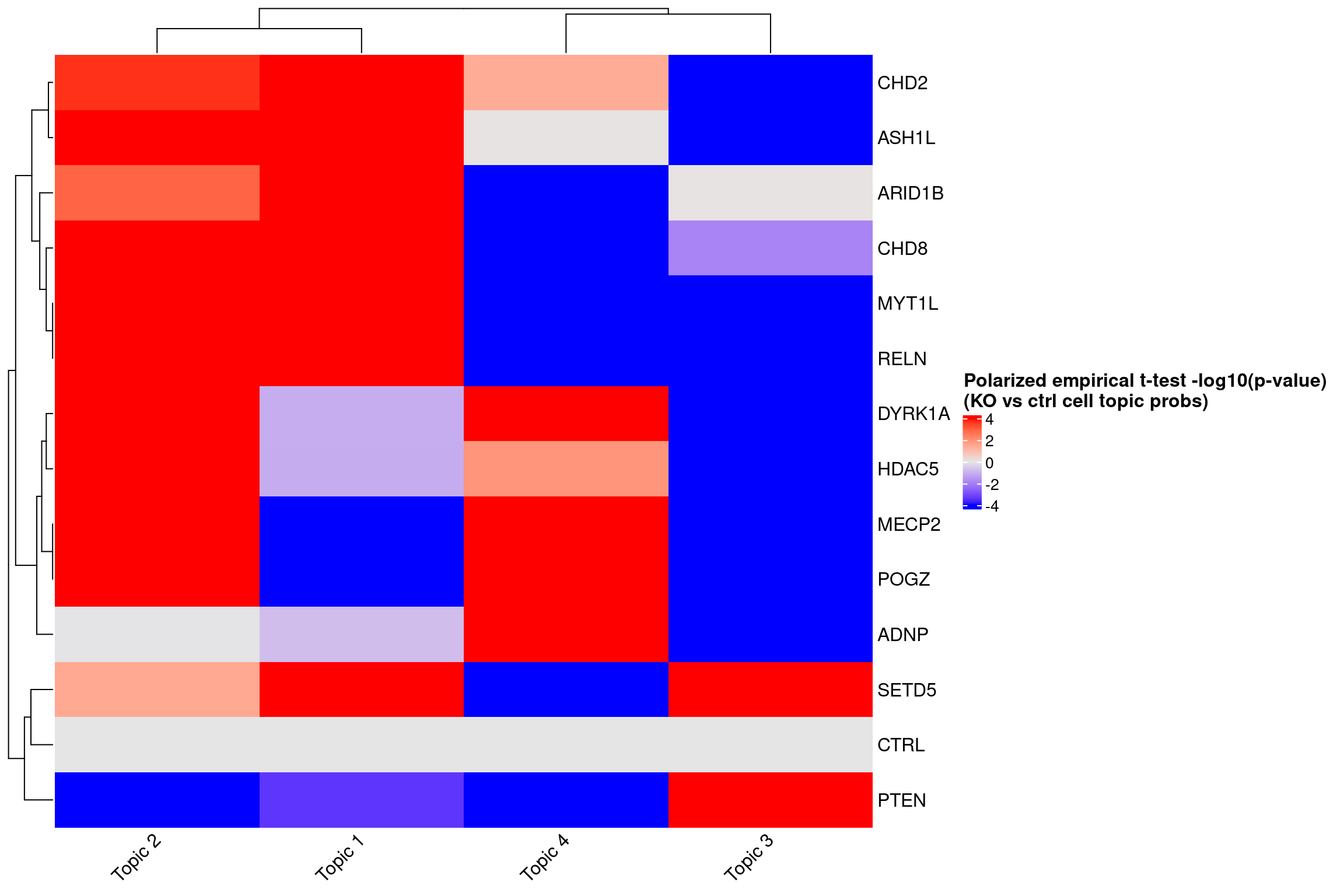
# dev.off()# pdf("music_output/music_merged_4_topics_empirical_tstats_fdr_dotplot.pdf",
# width = 12, height = 8)
KO_names <- rownames(fdr_mat)
dotplot_effectsize(t(effect_mat), t(fdr_mat),
reorder_markers = c(KO_names[KO_names!="CTRL"], "CTRL"),
color_lgd_title = "MUSIC T statistics",
size_lgd_title = "FDR",
max_score = 20,
min_score = -20,
by_score = 10) + coord_flip() +
theme(axis.text.x = element_text(angle = 45, vjust = 1))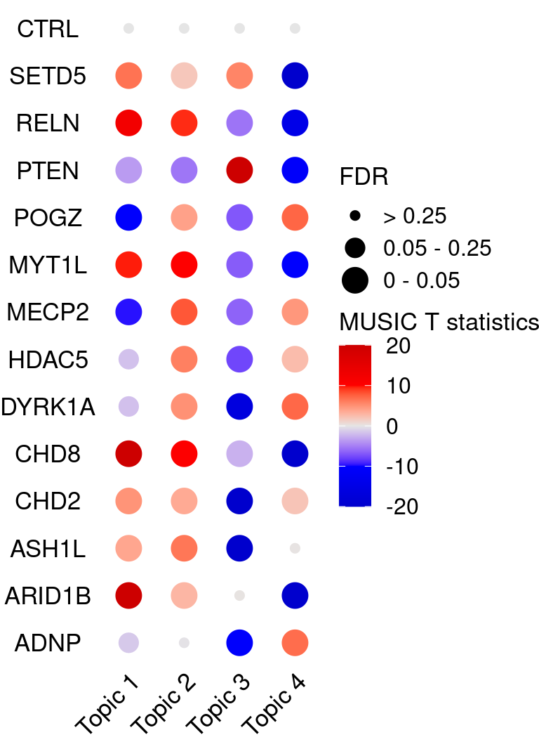
# dev.off()KO_names <- rownames(bonferroni_mat)
dotplot_effectsize(t(effect_mat), t(bonferroni_mat),
reorder_markers = c(KO_names[KO_names!="CTRL"], "CTRL"),
color_lgd_title = "MUSIC T statistics",
size_lgd_title = "Bonferroni\nadjusted p-value",
max_score = 20,
min_score = -20,
by_score = 10) +
coord_flip() +
theme(axis.text.x = element_text(angle = 45, vjust = 1))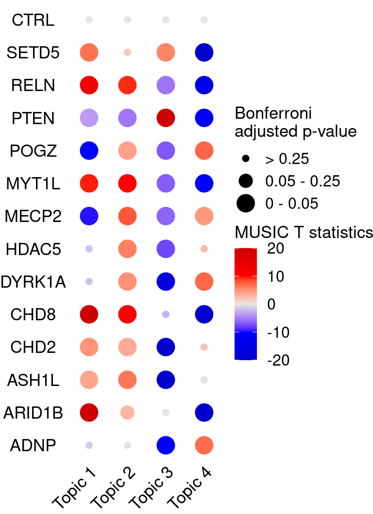
sessionInfo()R version 4.2.0 (2022-04-22)
Platform: x86_64-pc-linux-gnu (64-bit)
Running under: CentOS Linux 7 (Core)
Matrix products: default
BLAS/LAPACK: /software/openblas-0.3.13-el7-x86_64/lib/libopenblas_haswellp-r0.3.13.so
locale:
[1] LC_CTYPE=en_US.UTF-8 LC_NUMERIC=C LC_TIME=C
[4] LC_COLLATE=C LC_MONETARY=C LC_MESSAGES=C
[7] LC_PAPER=C LC_NAME=C LC_ADDRESS=C
[10] LC_TELEPHONE=C LC_MEASUREMENT=C LC_IDENTIFICATION=C
attached base packages:
[1] grid stats4 stats graphics grDevices utils datasets
[8] methods base
other attached packages:
[1] igraph_1.3.4 reshape2_1.4.4 gplots_3.1.3
[4] dplyr_1.0.9 lattice_0.20-45 ggplot2_3.3.6
[7] ComplexHeatmap_2.12.0 MUSIC_1.0 SAVER_1.1.3
[10] clusterProfiler_4.4.4 hash_2.2.6.2 topicmodels_0.2-12
[13] Biostrings_2.64.0 GenomeInfoDb_1.32.2 XVector_0.36.0
[16] IRanges_2.30.0 S4Vectors_0.34.0 BiocGenerics_0.42.0
[19] sp_1.4-7 SeuratObject_4.1.0 Seurat_4.1.1
[22] data.table_1.14.2 workflowr_1.7.0
loaded via a namespace (and not attached):
[1] scattermore_0.8 R.methodsS3_1.8.1 tidyr_1.2.0
[4] bit64_4.0.5 knitr_1.39 irlba_2.3.5
[7] R.utils_2.11.0 rpart_4.1.16 KEGGREST_1.36.2
[10] RCurl_1.98-1.7 doParallel_1.0.17 generics_0.1.2
[13] callr_3.7.0 cowplot_1.1.1 RSQLite_2.2.14
[16] shadowtext_0.1.2 RANN_2.6.1 future_1.25.0
[19] bit_4.0.4 enrichplot_1.16.2 spatstat.data_2.2-0
[22] xml2_1.3.3 httpuv_1.6.5 assertthat_0.2.1
[25] viridis_0.6.2 xfun_0.30 jquerylib_0.1.4
[28] evaluate_0.15 promises_1.2.0.1 fansi_1.0.3
[31] caTools_1.18.2 DBI_1.1.3 htmlwidgets_1.5.4
[34] spatstat.geom_2.4-0 purrr_0.3.4 ellipsis_0.3.2
[37] deldir_1.0-6 vctrs_0.4.1 Biobase_2.56.0
[40] Cairo_1.6-0 ROCR_1.0-11 abind_1.4-5
[43] cachem_1.0.6 withr_2.5.0 ggforce_0.3.4
[46] progressr_0.10.0 sctransform_0.3.3 treeio_1.20.2
[49] goftest_1.2-3 cluster_2.1.3 DOSE_3.22.1
[52] ape_5.6-2 lazyeval_0.2.2 crayon_1.5.1
[55] pkgconfig_2.0.3 slam_0.1-50 tweenr_1.0.2
[58] nlme_3.1-157 rlang_1.0.2 globals_0.15.0
[61] lifecycle_1.0.1 miniUI_0.1.1.1 downloader_0.4
[64] rprojroot_2.0.3 polyclip_1.10-0 matrixStats_0.62.0
[67] lmtest_0.9-40 Matrix_1.4-1 aplot_0.1.7
[70] zoo_1.8-10 whisker_0.4 ggridges_0.5.3
[73] GlobalOptions_0.1.2 processx_3.5.3 png_0.1-7
[76] viridisLite_0.4.0 rjson_0.2.21 bitops_1.0-7
[79] getPass_0.2-2 R.oo_1.24.0 KernSmooth_2.23-20
[82] blob_1.2.3 shape_1.4.6 stringr_1.4.0
[85] qvalue_2.28.0 parallelly_1.31.1 spatstat.random_2.2-0
[88] gridGraphics_0.5-1 scales_1.2.0 memoise_2.0.1
[91] magrittr_2.0.3 plyr_1.8.7 ica_1.0-2
[94] zlibbioc_1.42.0 compiler_4.2.0 scatterpie_0.1.8
[97] RColorBrewer_1.1-3 clue_0.3-61 fitdistrplus_1.1-8
[100] cli_3.3.0 listenv_0.8.0 patchwork_1.1.1
[103] pbapply_1.5-0 ps_1.7.0 MASS_7.3-56
[106] mgcv_1.8-40 tidyselect_1.1.2 stringi_1.7.6
[109] highr_0.9 yaml_2.3.5 GOSemSim_2.22.0
[112] ggrepel_0.9.1 sass_0.4.1 fastmatch_1.1-3
[115] tools_4.2.0 future.apply_1.9.0 parallel_4.2.0
[118] circlize_0.4.15 rstudioapi_0.13 foreach_1.5.2
[121] git2r_0.30.1 gridExtra_2.3 farver_2.1.0
[124] Rtsne_0.16 ggraph_2.0.6 digest_0.6.29
[127] rgeos_0.5-9 shiny_1.7.1 Rcpp_1.0.8.3
[130] later_1.3.0 RcppAnnoy_0.0.19 httr_1.4.3
[133] AnnotationDbi_1.58.0 colorspace_2.0-3 fs_1.5.2
[136] tensor_1.5 reticulate_1.24 splines_4.2.0
[139] uwot_0.1.11 yulab.utils_0.0.5 tidytree_0.4.0
[142] spatstat.utils_2.3-1 graphlayouts_0.8.1 ggplotify_0.1.0
[145] plotly_4.10.0 xtable_1.8-4 jsonlite_1.8.0
[148] ggtree_3.4.2 tidygraph_1.2.2 NLP_0.2-1
[151] modeltools_0.2-23 ggfun_0.0.7 R6_2.5.1
[154] tm_0.7-8 pillar_1.7.0 htmltools_0.5.2
[157] mime_0.12 glue_1.6.2 fastmap_1.1.0
[160] BiocParallel_1.30.3 codetools_0.2-18 fgsea_1.22.0
[163] utf8_1.2.2 bslib_0.3.1 spatstat.sparse_2.1-1
[166] tibble_3.1.7 leiden_0.4.2 gtools_3.9.2
[169] GO.db_3.15.0 survival_3.3-1 rmarkdown_2.14
[172] munsell_0.5.0 DO.db_2.9 GetoptLong_1.0.5
[175] GenomeInfoDbData_1.2.8 iterators_1.0.14 gtable_0.3.0
[178] spatstat.core_2.4-2