DNase footprint profiles using ENCODE DNase-seq data

Last updated: 2018-08-30

workflowr checks: (Click a bullet for more information)

✔ R Markdown file: up-to-date

Great! Since the R Markdown file has been committed to the Git repository, you know the exact version of the code that produced these results.
✔ Environment: empty

Great job! The global environment was empty. Objects defined in the global environment can affect the analysis in your R Markdown file in unknown ways. For reproduciblity it’s best to always run the code in an empty environment.
✔ Seed: set.seed(20180613)

The command set.seed(20180613) was run prior to running the code in the R Markdown file. Setting a seed ensures that any results that rely on randomness, e.g. subsampling or permutations, are reproducible.
✔ Session information: recorded

Great job! Recording the operating system, R version, and package versions is critical for reproducibility.

✔ Repository version: e17a41f

Great! You are using Git for version control. Tracking code development and connecting the code version to the results is critical for reproducibility. The version displayed above was the version of the Git repository at the time these results were generated.

Note that you need to be careful to ensure that all relevant files for the analysis have been committed to Git prior to generating the results (you can use wflow_publish or wflow_git_commit). workflowr only checks the R Markdown file, but you know if there are other scripts or data files that it depends on. Below is the status of the Git repository when the results were generated:


Ignored files:
    Ignored:    .DS_Store
    Ignored:    .Rhistory
    Ignored:    .Rproj.user/
    Ignored:    code_RCC/.DS_Store
    Ignored:    data/.DS_Store

Untracked files:
    Untracked:  analysis/ATACseq_footprint_profiles_GGR_Duke.Rmd
    Untracked:  analysis/ATACseq_footprint_profiles_OliviaGray.Rmd
    Untracked:  analysis/ATACseq_footprint_profiles_OliviaGray_HAEC.Rmd
    Untracked:  analysis/ATACseq_preprocessing_pipeline_GGR_hg38.Rmd
    Untracked:  code_RCC/update_bamnames.R
    Untracked:  docs/figure/ATACseq_footprint_profiles_GGR_Duke.Rmd/
    Untracked:  workflow_setup.R

Unstaged changes:
    Modified:   analysis/ATACseq_preprocessing_pipeline.Rmd
    Modified:   analysis/index.Rmd
    Modified:   code_RCC/fimo_jaspar_motif_rcc.sh
    Modified:   code_RCC/genome_coverage_bamToBigwig_GGR_hg38.sh
    Modified:   code_RCC/get_motif_count_matrices_GGR_hg38.sh

Note that any generated files, e.g. HTML, png, CSS, etc., are not included in this status report because it is ok for generated content to have uncommitted changes.

Expand here to see past versions:

File	Version	Author	Date	Message
Rmd	e17a41f	kevinlkx	2018-08-30	plot DNase footprint profiles of CTCF and REST using ENCODE data
html	fdc07be	kevinlkx	2018-08-30	Build site.
Rmd	2783ac9	kevinlkx	2018-08-30	plot DNase footprint profiles of CTCF and REST using ENCODE data
html	dcc47c4	kevinlkx	2018-08-29	Build site.
Rmd	eed77b5	kevinlkx	2018-08-29	plot DNase footprint profiles of CTCF and REST using ENCODE data
html	7adcba7	kevinlkx	2018-08-29	Build site.
Rmd	ed49eff	kevinlkx	2018-08-29	plot DNase footprint profiles of CTCF and REST using ENCODE data
html	57479c5	kevinlkx	2018-08-29	Build site.
Rmd	bb65514	kevinlkx	2018-08-29	plot DNase footprint profiles of CTCF and REST using ENCODE data
html	98209cf	kevinlkx	2018-08-29	Build site.
Rmd	2f894eb	kevinlkx	2018-08-29	plot DNase footprint profiles of CTCF and REST using ENCODE data
html	0e20593	kevinlkx	2018-08-29	Build site.
Rmd	a233f11	kevinlkx	2018-08-29	plot DNase footprint profiles of CTCF and REST using ENCODE data
html	b182c05	kevinlkx	2018-08-29	Build site.
Rmd	09836f9	kevinlkx	2018-08-29	plot DNase footprint profiles of CTCF and REST using ENCODE data
html	35c5feb	kevinlkx	2018-08-29	Build site.
Rmd	f318dd5	kevinlkx	2018-08-29	plot DNase footprint profiles of CTCF and REST using ENCODE data

functions

##### Functions #####
## load and combine count matrices
load_combine_counts <- function(tf_name, pwm_name, dir_count_matrix){
  cat("Loading count matrices ... \n")
  counts_fwd.df <- read.table(paste0(dir_count_matrix, "/", tf_name, "/", pwm_name, "_hg19_dnase_fwdcounts.m.gz"))
  counts_rev.df <- read.table(paste0(dir_count_matrix, "/", tf_name, "/", pwm_name, "_hg19_dnase_revcounts.m.gz"))
  
  ## the first 5 columns from "bwtool extract" are chr, start, end, name, and the number of data points
  counts_fwd.df <- counts_fwd.df[, -c(1:5)]
  counts_rev.df <- counts_rev.df[, -c(1:5)]
  
  colnames(counts_fwd.df) <- paste0("fwd", 1:ncol(counts_fwd.df))
  colnames(counts_rev.df) <- paste0("rev", 1:ncol(counts_rev.df))
  
  counts_combined.m <- as.matrix(cbind(counts_fwd.df, counts_rev.df))
  
  return(counts_combined.m)
}

## select candidate sites by mapability and PWM score cutoffs
select_sites <- function(sites.df, thresh_mapability=NULL, thresh_PWMscore=NULL, readstats_name=NULL){
  #  cat("loading sites ...\n")
  cat("Select candidate sites \n")
  
  if(!is.null(thresh_mapability) || !is.na(thresh_mapability)){
    cat("Select candidate sites with mapability >=", thresh_mapability, "\n")
    idx_mapability <- (sites.df[,"mapability"] >= thresh_mapability)
  }else{
    idx_mapability <- rep(TRUE, nrow(sites.df))
  }
  
  if(!is.null(thresh_PWMscore) || !is.na(thresh_PWMscore)){
    cat("Select candidate sites with PWM score >=", thresh_PWMscore, "\n")
    idx_pwm <- (sites.df[,"pwm_score"] >= thresh_PWMscore)
  }else{
    idx_pwm <- rep(TRUE, nrow(sites.df))
  }
  
  if(!is.null(readstats_name)){
    readstats.df <- read.table(readstats_name, header = F)
    ## if the readstats.df contains chrY, then it means the cell type is male, then the candidate sites should contain chrY,
    ## otherwise, the cell type is female, then the candidate sites on chrY should be removed.
    if( "chrY" %in% readstats.df[,1] ){
      cat("include chrY sites \n")
      idx_chr <- (sites.df[,1] != "")
    }else{
      cat("chrY NOT in the bam file, filter out chrY sites \n")
      ## remove chrY from candidate (motif) sites
      idx_chr <- (sites.df[,1] != "chrY")
    }
    
  }else{
    idx_chr <- rep(TRUE, nrow(sites.df))
  }
  
  idx_select <- which(idx_mapability & idx_pwm & idx_chr)
  
  return(idx_select)
}

parameters

ver_genome <- "hg19"
flank <- 100
thresh_mapability <- 0.8
thresh_PWMscore <- 10
num_top_sites <- 1000 # plot top sites
max_cuts <- 20 # Clip extreme values
dir_data <- "~/Dropbox/research/ATAC_DNase/"

CTCF in GM12878 cell type

load DNase footprint data

cell_type <- "GM12878"
tf_name <- "CTCF"
pwm_name <- "CTCF_MA0139.1_1e-5"

dir_count_matrix <- paste0(dir_data, "/DNase-seq_ENCODE/", cell_type, "/DNaseSeq/DNase_tagcount_matrix/")
dir_sites_chip <- paste0(dir_data, "/DNase-seq_ENCODE/", cell_type, "/ChIPSeq/")

filename_sites <- paste0(dir_sites_chip, "/", "chipseq_", cell_type, "_", pwm_name, "_flank", flank, "_exp1.totalcount")

sites.df <- read.table(filename_sites, header = T, comment.char = "!", stringsAsFactors = F)
sites.df <- sites.df[, c("chr", "start", "end", "site", "pwmScore", "strand", "pValue", "mapability", "ChIP_mean")]
colnames(sites.df) = c("chr", "start", "end", "name", "pwm_score", "strand", "p_value", "mapability", "ChIP")

idx_select <- select_sites(sites.df, thresh_mapability, thresh_PWMscore)

Select candidate sites 
Select candidate sites with mapability >= 0.8 
Select candidate sites with PWM score >= 10

sites.df <- sites.df[idx_select, ]
cat("Number of sites:", nrow(sites.df), "\n")

Number of sites: 54859

counts_combined.m <- load_combine_counts(tf_name, pwm_name, dir_count_matrix)

Loading count matrices ...

counts_combined.m <- counts_combined.m[idx_select,]

## Clip extreme values
counts_combined.m[counts_combined.m > max_cuts] <- max_cuts

cat("Dimension of", dim(counts_combined.m), "\n")

Dimension of 54859 436

if(nrow(counts_combined.m) != nrow(sites.df)){
  stop("Sites not matched!")
}

plot footprint profiles of highest occupancy

order_selected <- order(sites.df$ChIP, decreasing = T)[1:num_top_sites]
counts_selected.m <- counts_combined.m[order_selected,]
counts_profile <- apply(counts_selected.m, 2, mean)

par(mfrow = c(1,2))
counts <- counts_profile[1:(length(counts_profile)/2)]
plot(counts, type = "l", col = "blue", xlab = "Relative position (bp)", ylab = "Average counts", 
     main = "", xaxt = "n")
mtext(text = paste(tf_name, cell_type, "forward strand"), side = 3, line = 1, cex = 1)
axis(1,at=c(1, flank+1, length(counts)-flank, length(counts)), labels=c(-flank, '','' ,flank), 
     cex.axis = 1, tck=-0.03, tick = T, cex = 1)

counts <- counts_profile[(length(counts_profile)/2+1): length(counts_profile)]

plot(counts, type = "l", col = "red", xlab = "Relative position (bp)", ylab = "Average counts", 
     main = "", xaxt = "n")
mtext(text = paste(tf_name, cell_type, "reverse strand"), side = 3, line = 1, cex = 1)
axis(1,at=c(1, flank+1, length(counts)-flank, length(counts)), labels=c(-flank, '','' ,flank), 
     cex.axis = 1, tck=-0.03, tick = T, cex = 1)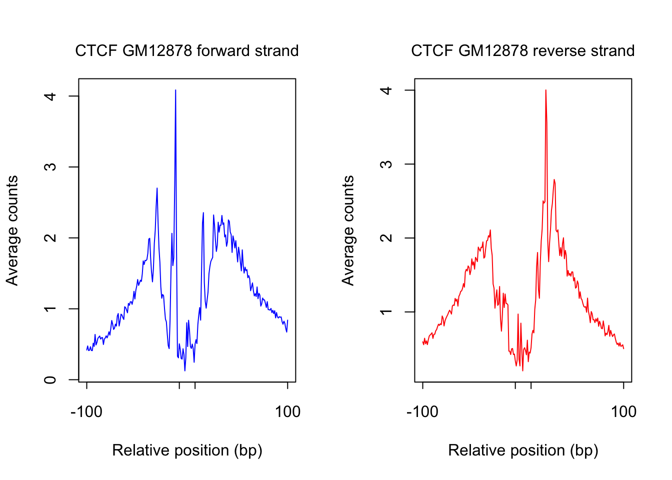

Expand here to see past versions of unnamed-chunk-4-1.png:

Version	Author	Date
35c5feb	kevinlkx	2018-08-29

## save counts matrix
dir_matrix_examples <- paste0(dir_data, "/DNase-seq_ENCODE/", cell_type, "/DNaseSeq/DNase_count_matrix_examples/")
dir.create(dir_matrix_examples, showWarnings = F, recursive = T)
saveRDS(counts_selected.m, paste0(dir_matrix_examples, "/", pwm_name, "_", cell_type, "_dnase_counts_selected_sites.rds"))

plot footprint profiles of most accessible sites

order_selected <- order(rowSums(counts_combined.m), decreasing = T)[1:num_top_sites]
counts_selected.m <- counts_combined.m[order_selected,]
counts_profile <- apply(counts_selected.m, 2, mean)

par(mfrow = c(1,2))
counts <- counts_profile[1:(length(counts_profile)/2)]
plot(counts, type = "l", col = "blue", xlab = "Relative position (bp)", ylab = "Average counts", 
     main = "", xaxt = "n")
mtext(text = paste(tf_name, cell_type, "forward strand"), side = 3, line = 1, cex = 1)
axis(1,at=c(1, flank+1, length(counts)-flank, length(counts)), labels=c(-flank, '','' ,flank), 
     cex.axis = 1, tck=-0.03, tick = T, cex = 1)

counts <- counts_profile[(length(counts_profile)/2+1): length(counts_profile)]

plot(counts, type = "l", col = "red", xlab = "Relative position (bp)", ylab = "Average counts", 
     main = "", xaxt = "n")
mtext(text = paste(tf_name, cell_type, "reverse strand"), side = 3, line = 1, cex = 1)
axis(1,at=c(1, flank+1, length(counts)-flank, length(counts)), labels=c(-flank, '','' ,flank), 
     cex.axis = 1, tck=-0.03, tick = T, cex = 1)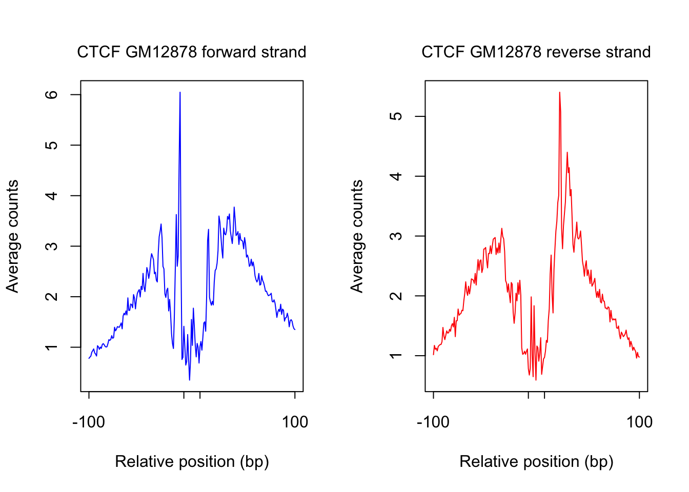

Expand here to see past versions of unnamed-chunk-5-1.png:

Version	Author	Date
35c5feb	kevinlkx	2018-08-29

CTCF in K562 cell type

load DNase footprint data

cell_type <- "K562"
tf_name <- "CTCF"
pwm_name <- "CTCF_MA0139.1_1e-5"

dir_count_matrix <- paste0(dir_data, "/DNase-seq_ENCODE/", cell_type, "/DNaseSeq/DNase_tagcount_matrix/")
dir_sites_chip <- paste0(dir_data, "/DNase-seq_ENCODE/", cell_type, "/ChIPSeq/")

filename_sites <- paste0(dir_sites_chip, "/", "chipseq_", cell_type, "_", pwm_name, "_flank", flank, "_exp1.totalcount")

sites.df <- read.table(filename_sites, header = T, comment.char = "!", stringsAsFactors = F)
sites.df <- sites.df[, c("chr", "start", "end", "site", "pwmScore", "strand", "pValue", "mapability", "ChIP_mean")]
colnames(sites.df) = c("chr", "start", "end", "name", "pwm_score", "strand", "p_value", "mapability", "ChIP")

idx_select <- select_sites(sites.df, thresh_mapability, thresh_PWMscore)

Select candidate sites 
Select candidate sites with mapability >= 0.8 
Select candidate sites with PWM score >= 10

sites.df <- sites.df[idx_select, ]
cat("Number of sites:", nrow(sites.df), "\n")

Number of sites: 54859

counts_combined.m <- load_combine_counts(tf_name, pwm_name, dir_count_matrix)

Loading count matrices ...

counts_combined.m <- counts_combined.m[idx_select,]

## Clip extreme values
counts_combined.m[counts_combined.m > max_cuts] <- max_cuts

cat("Dimension of", dim(counts_combined.m), "\n")

Dimension of 54859 436

if(nrow(counts_combined.m) != nrow(sites.df)){
  stop("Sites not matched!")
}

plot footprint profiles of highest occupancy sites

order_selected <- order(sites.df$ChIP, decreasing = T)[1:num_top_sites]
counts_selected.m <- counts_combined.m[order_selected,]
counts_profile <- apply(counts_selected.m, 2, mean)

par(mfrow = c(1,2))
counts <- counts_profile[1:(length(counts_profile)/2)]
plot(counts, type = "l", col = "blue", xlab = "Relative position (bp)", ylab = "Average counts", 
     main = "", xaxt = "n")
mtext(text = paste(tf_name, cell_type, "forward strand"), side = 3, line = 1, cex = 1)
axis(1,at=c(1, flank+1, length(counts)-flank, length(counts)), labels=c(-flank, '','' ,flank), 
     cex.axis = 1, tck=-0.03, tick = T, cex = 1)

counts <- counts_profile[(length(counts_profile)/2+1): length(counts_profile)]

plot(counts, type = "l", col = "red", xlab = "Relative position (bp)", ylab = "Average counts", 
     main = "", xaxt = "n")
mtext(text = paste(tf_name, cell_type, "reverse strand"), side = 3, line = 1, cex = 1)
axis(1,at=c(1, flank+1, length(counts)-flank, length(counts)), labels=c(-flank, '','' ,flank), 
     cex.axis = 1, tck=-0.03, tick = T, cex = 1)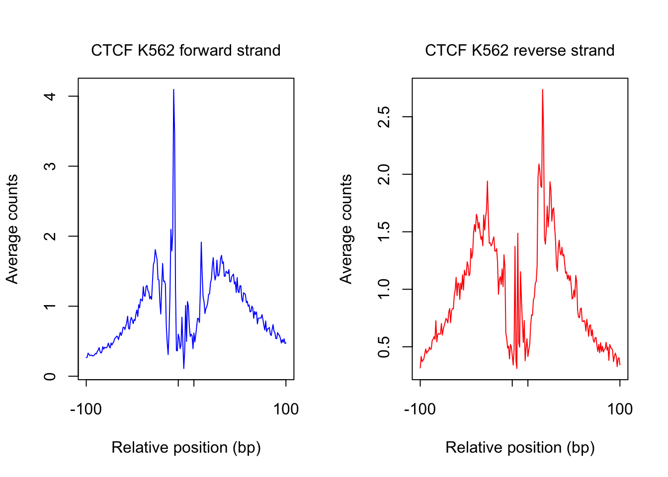

Expand here to see past versions of unnamed-chunk-7-1.png:

Version	Author	Date
35c5feb	kevinlkx	2018-08-29

## save counts matrix
dir_matrix_examples <- paste0(dir_data, "/DNase-seq_ENCODE/", cell_type, "/DNaseSeq/DNase_count_matrix_examples/")
dir.create(dir_matrix_examples, showWarnings = F, recursive = T)
saveRDS(counts_selected.m, paste0(dir_matrix_examples, "/", pwm_name, "_", cell_type, "_dnase_counts_selected_sites.rds"))

REST in GM12878 cell type

load DNase footprint data

cell_type <- "GM12878"
tf_name <- "REST"
pwm_name <- "REST_MA0138.2_1e-5"

dir_count_matrix <- paste0(dir_data, "/DNase-seq_ENCODE/", cell_type, "/DNaseSeq/DNase_tagcount_matrix/")
dir_sites_chip <- paste0(dir_data, "/DNase-seq_ENCODE/", cell_type, "/ChIPSeq/")

filename_sites <- paste0(dir_sites_chip, "/", "chipseq_", cell_type, "_", pwm_name, "_flank", flank, "_exp1.totalcount")

sites.df <- read.table(filename_sites, header = T, comment.char = "!", stringsAsFactors = F)
sites.df <- sites.df[, c("chr", "start", "end", "site", "pwmScore", "strand", "pValue", "mapability", "ChIP_mean")]
colnames(sites.df) = c("chr", "start", "end", "name", "pwm_score", "strand", "p_value", "mapability", "ChIP")

idx_select <- select_sites(sites.df, thresh_mapability, thresh_PWMscore)

Select candidate sites 
Select candidate sites with mapability >= 0.8 
Select candidate sites with PWM score >= 10

sites.df <- sites.df[idx_select, ]
cat("Number of sites:", nrow(sites.df), "\n")

Number of sites: 54533

counts_combined.m <- load_combine_counts(tf_name, pwm_name, dir_count_matrix)

Loading count matrices ...

counts_combined.m <- counts_combined.m[idx_select,]

## Clip extreme values
counts_combined.m[counts_combined.m > max_cuts] <- max_cuts

cat("Dimension of", dim(counts_combined.m), "\n")

Dimension of 54533 440

if(nrow(counts_combined.m) != nrow(sites.df)){
  stop("Sites not matched!")
}

plot footprint profiles of highest occupancy sites

order_selected <- order(sites.df$ChIP, decreasing = T)[1:num_top_sites]
counts_selected.m <- counts_combined.m[order_selected,]
counts_profile <- apply(counts_selected.m, 2, mean)

par(mfrow = c(1,2))
counts <- counts_profile[1:(length(counts_profile)/2)]
plot(counts, type = "l", col = "blue", xlab = "Relative position (bp)", ylab = "Average counts", 
     main = "", xaxt = "n")
mtext(text = paste(tf_name, cell_type, "forward strand"), side = 3, line = 1, cex = 1)
axis(1,at=c(1, flank+1, length(counts)-flank, length(counts)), labels=c(-flank, '','' ,flank), 
     cex.axis = 1, tck=-0.03, tick = T, cex = 1)

counts <- counts_profile[(length(counts_profile)/2+1): length(counts_profile)]

plot(counts, type = "l", col = "red", xlab = "Relative position (bp)", ylab = "Average counts", 
     main = "", xaxt = "n")
mtext(text = paste(tf_name, cell_type, "reverse strand"), side = 3, line = 1, cex = 1)
axis(1,at=c(1, flank+1, length(counts)-flank, length(counts)), labels=c(-flank, '','' ,flank), 
     cex.axis = 1, tck=-0.03, tick = T, cex = 1)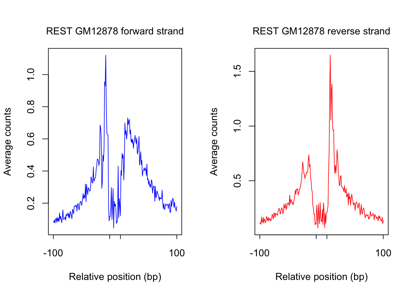

Expand here to see past versions of unnamed-chunk-9-1.png:

Version	Author	Date
0e20593	kevinlkx	2018-08-29

## save counts matrix
dir_matrix_examples <- paste0(dir_data, "/DNase-seq_ENCODE/", cell_type, "/DNaseSeq/DNase_count_matrix_examples/")
dir.create(dir_matrix_examples, showWarnings = F, recursive = T)
saveRDS(counts_selected.m, paste0(dir_matrix_examples, "/", pwm_name, "_", cell_type, "_dnase_counts_selected_sites.rds"))

plot footprint profiles of most accessible sites

order_selected <- order(rowSums(counts_combined.m), decreasing = T)[1:num_top_sites]
counts_selected.m <- counts_combined.m[order_selected,]
counts_profile <- apply(counts_selected.m, 2, mean)

par(mfrow = c(1,2))
counts <- counts_profile[1:(length(counts_profile)/2)]
plot(counts, type = "l", col = "blue", xlab = "Relative position (bp)", ylab = "Average counts", 
     main = "", xaxt = "n")
mtext(text = paste(tf_name, cell_type, "forward strand"), side = 3, line = 1, cex = 1)
axis(1,at=c(1, flank+1, length(counts)-flank, length(counts)), labels=c(-flank, '','' ,flank), 
     cex.axis = 1, tck=-0.03, tick = T, cex = 1)

counts <- counts_profile[(length(counts_profile)/2+1): length(counts_profile)]

plot(counts, type = "l", col = "red", xlab = "Relative position (bp)", ylab = "Average counts", 
     main = "", xaxt = "n")
mtext(text = paste(tf_name, cell_type, "reverse strand"), side = 3, line = 1, cex = 1)
axis(1,at=c(1, flank+1, length(counts)-flank, length(counts)), labels=c(-flank, '','' ,flank), 
     cex.axis = 1, tck=-0.03, tick = T, cex = 1)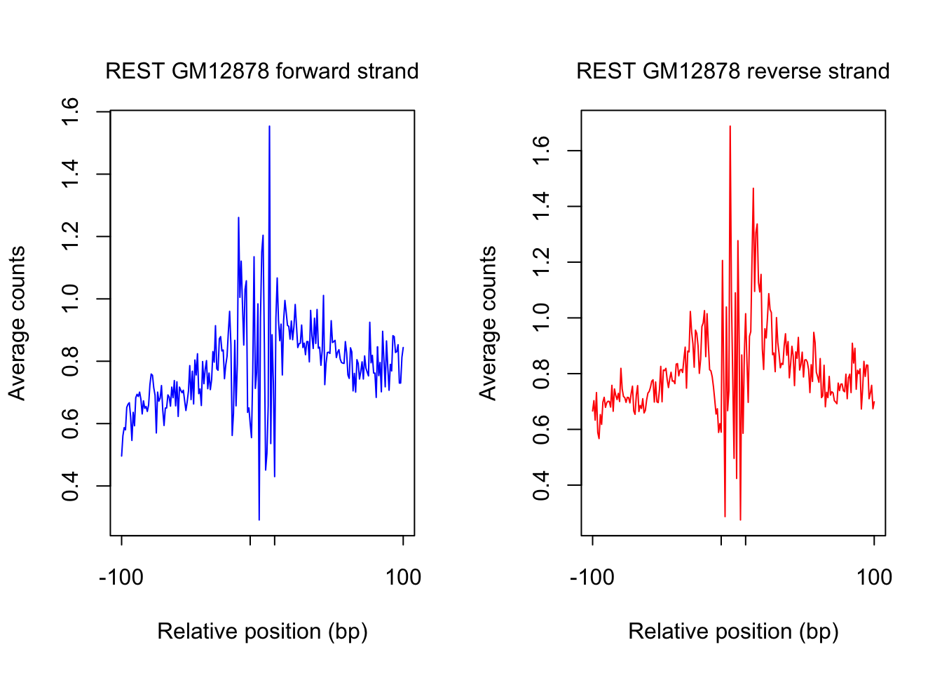

Expand here to see past versions of unnamed-chunk-10-1.png:

Version	Author	Date
0e20593	kevinlkx	2018-08-29
35c5feb	kevinlkx	2018-08-29

REST in K562 cell type

load DNase footprint data

cell_type <- "K562"
tf_name <- "REST"
pwm_name <- "REST_MA0138.2_1e-5"

dir_count_matrix <- paste0(dir_data, "/DNase-seq_ENCODE/", cell_type, "/DNaseSeq/DNase_tagcount_matrix/")
dir_sites_chip <- paste0(dir_data, "/DNase-seq_ENCODE/", cell_type, "/ChIPSeq/")

filename_sites <- paste0(dir_sites_chip, "/", "chipseq_", cell_type, "_", pwm_name, "_flank", flank, "_exp1.totalcount")

sites.df <- read.table(filename_sites, header = T, comment.char = "!", stringsAsFactors = F)
sites.df <- sites.df[, c("chr", "start", "end", "site", "pwmScore", "strand", "pValue", "mapability", "ChIP_mean")]
colnames(sites.df) = c("chr", "start", "end", "name", "pwm_score", "strand", "p_value", "mapability", "ChIP")

idx_select <- select_sites(sites.df, thresh_mapability, thresh_PWMscore)

Select candidate sites 
Select candidate sites with mapability >= 0.8 
Select candidate sites with PWM score >= 10

sites.df <- sites.df[idx_select, ]
cat("Number of sites:", nrow(sites.df), "\n")

Number of sites: 54533

counts_combined.m <- load_combine_counts(tf_name, pwm_name, dir_count_matrix)

Loading count matrices ...

counts_combined.m <- counts_combined.m[idx_select,]

## Clip extreme values
counts_combined.m[counts_combined.m > max_cuts] <- max_cuts

cat("Dimension of", dim(counts_combined.m), "\n")

Dimension of 54533 440

if(nrow(counts_combined.m) != nrow(sites.df)){
  stop("Sites not matched!")
}

plot footprint profiles of highest occupancy sites

order_selected <- order(sites.df$ChIP, decreasing = T)[1:num_top_sites]
counts_selected.m <- counts_combined.m[order_selected,]
counts_profile <- apply(counts_selected.m, 2, mean)


par(mfrow = c(1,2))
counts <- counts_profile[1:(length(counts_profile)/2)]
plot(counts, type = "l", col = "blue", xlab = "Relative position (bp)", ylab = "Average counts", 
     main = "", xaxt = "n")
mtext(text = paste(tf_name, cell_type, "forward strand"), side = 3, line = 1, cex = 1)
axis(1,at=c(1, flank+1, length(counts)-flank, length(counts)), labels=c(-flank, '','' ,flank), 
     cex.axis = 1, tck=-0.03, tick = T, cex = 1)

counts <- counts_profile[(length(counts_profile)/2+1): length(counts_profile)]

plot(counts, type = "l", col = "red", xlab = "Relative position (bp)", ylab = "Average counts", 
     main = "", xaxt = "n")
mtext(text = paste(tf_name, cell_type, "reverse strand"), side = 3, line = 1, cex = 1)
axis(1,at=c(1, flank+1, length(counts)-flank, length(counts)), labels=c(-flank, '','' ,flank), 
     cex.axis = 1, tck=-0.03, tick = T, cex = 1)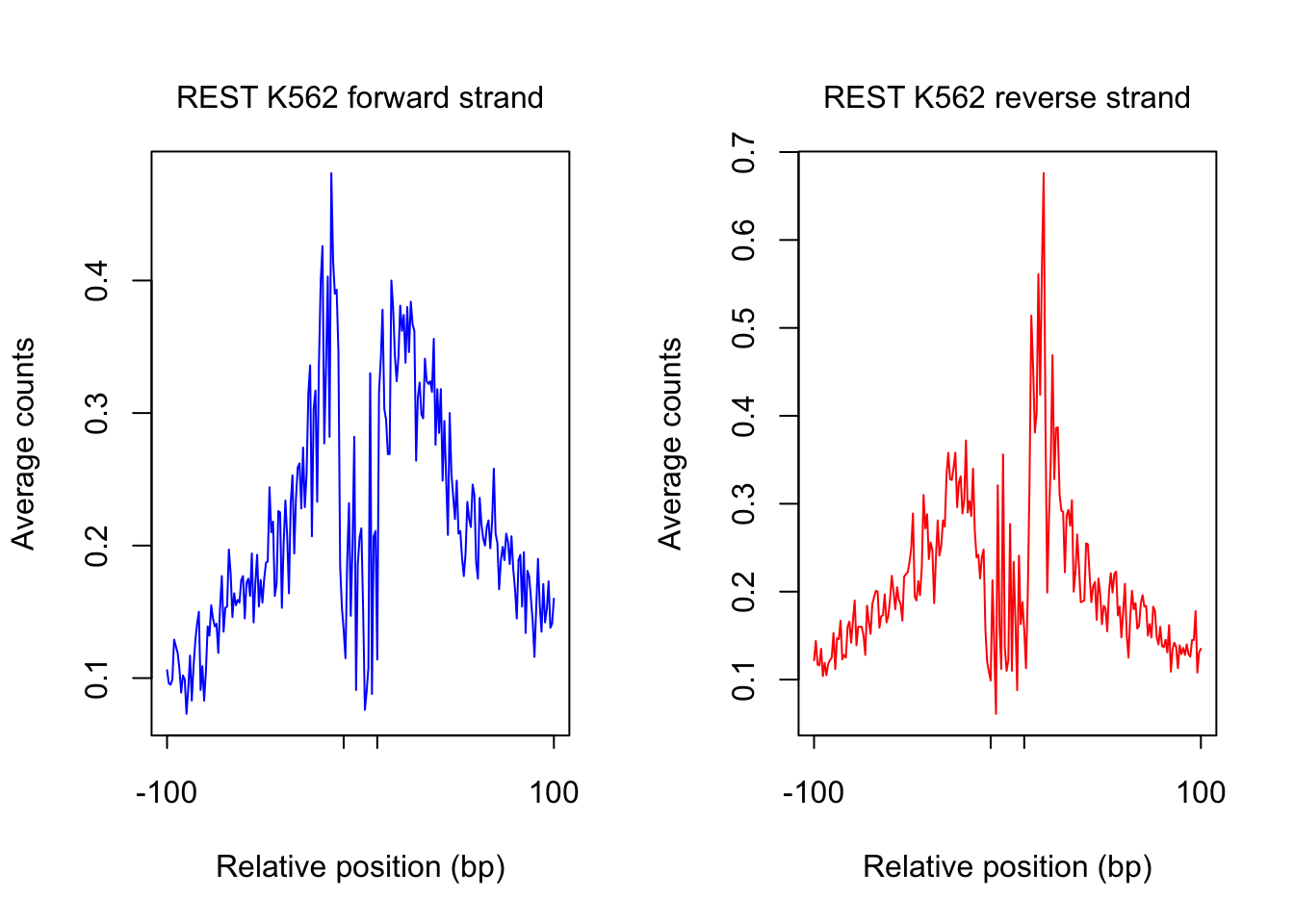

Expand here to see past versions of unnamed-chunk-12-1.png:

Version	Author	Date
0e20593	kevinlkx	2018-08-29

## save counts matrix
dir_matrix_examples <- paste0(dir_data, "/DNase-seq_ENCODE/", cell_type, "/DNaseSeq/DNase_count_matrix_examples/")
dir.create(dir_matrix_examples, showWarnings = F, recursive = T)
saveRDS(counts_selected.m, paste0(dir_matrix_examples, "/", pwm_name, "_", cell_type, "_dnase_counts_selected_sites.rds"))

Session information

sessionInfo()

R version 3.4.3 (2017-11-30)
Platform: x86_64-apple-darwin15.6.0 (64-bit)
Running under: macOS High Sierra 10.13.6

Matrix products: default
BLAS: /Library/Frameworks/R.framework/Versions/3.4/Resources/lib/libRblas.0.dylib
LAPACK: /Library/Frameworks/R.framework/Versions/3.4/Resources/lib/libRlapack.dylib

locale:
[1] en_US.UTF-8/en_US.UTF-8/en_US.UTF-8/C/en_US.UTF-8/en_US.UTF-8

attached base packages:
[1] stats     graphics  grDevices utils     datasets  methods   base     

loaded via a namespace (and not attached):
 [1] workflowr_1.1.1   Rcpp_0.12.16      digest_0.6.15    
 [4] rprojroot_1.3-2   R.methodsS3_1.7.1 backports_1.1.2  
 [7] git2r_0.21.0      magrittr_1.5      evaluate_0.10.1  
[10] stringi_1.1.7     whisker_0.3-2     R.oo_1.22.0      
[13] R.utils_2.6.0     rmarkdown_1.9     tools_3.4.3      
[16] stringr_1.3.0     yaml_2.1.18       compiler_3.4.3   
[19] htmltools_0.3.6   knitr_1.20

This reproducible R Markdown analysis was created with workflowr 1.1.1

DNase footprint profiles using ENCODE DNase-seq data

Kaixuan Luo

7/31/2018

functions

parameters

CTCF in GM12878 cell type

load DNase footprint data

plot footprint profiles of highest occupancy

plot footprint profiles of most accessible sites

CTCF in K562 cell type

load DNase footprint data

plot footprint profiles of highest occupancy sites

REST in GM12878 cell type

load DNase footprint data

plot footprint profiles of highest occupancy sites

plot footprint profiles of most accessible sites

REST in K562 cell type

load DNase footprint data

plot footprint profiles of highest occupancy sites

Session information